American Journal of Plant Sciences
Vol.5 No.4(2014), Article ID:43250,6 pages DOI:10.4236/ajps.2014.54057
Dependence of the Plant Productivity on Optimal Food Regime and Density
Institute of Soil Science and Agrochemistry of НАН of Azerbaijan, Baku, Azerbaijan.
Email: *naila.56@mail.ru
Copyright © 2014 N. İ. Orudzheva et al. This is an open access article distributed under the Creative Commons Attribution License, which permits unrestricted use, distribution, and reproduction in any medium, provided the original work is properly cited. In accordance of the Creative Commons Attribution License all Copyrights © 2014 are reserved for SCIRP and the owner of the intellectual property N. İ. Orudzheva et al. All Copyright © 2014 are guarded by law and by SCIRP as a guardian.
Received December 5th, 2013; revised January 6th, 2014; accepted January 16th, 2014
KEYWORDS
Standing Density; Vegetable Crops; Approximation; Yield; Mineral Fertilizers; Nutrition Mode; Nutrients; Diffusion; Linear Approximation; The Cubic Approximation
ABSTRACT
It has been studied the dependence of vegetable crop yield on standing density of the plant. Field experiments have been conducted on plain Mughan of Azerbaijan Republic. For identifying the maximum value of crop yield it has been carried out approximation of the results of field works with special programs. The point of yield maximum for tomatoes, eggplant, and peppers has been calculated, and also it has been carried out the variation in the amount of nitrogen to decreasing direction in nutrition circuit and the impact of this variation on yield has been regarded. The obtained data are interpreted on the basis of two-substrate model of plant growth.
1. Introduction
Dependence between the yield Y, kg/m2 and standing density ρ (quantity per 1 m2) is an important question of well-deserved attention [1,2]. For some crops it is expedient to take into account not just the scalar standing density ρ and also the distance between seeds in a row S, and width of interrow S2. Berrke [3], for example proposes to consider the perpendicularity of location of plants to the row direction by means of the expression.
 (1)
(1)
where ω: mass of plants, : yield, а:
 .
.
It should be noted, that within the functionalistic approach the area A, m2 attributable to each plant is defined as
 (2)
(2)
And in this case it is implied that the volume m3 of soil attributable to each plant equals
 (3)
(3)
Formulas (2) and (3) should be regarded only as the first approach to the adequate description of a difficult situation). It should be noted that if “density” of ρ standing increases due to “capture” the emptiness between “own” soil volumes of plants, the dependence of crop yield on density of standing has a rectilinear form [4]. The maximum yield is obtained at such values of standing density when the level of “confrontation” of the plant with their “close” neighbors gets a minimum value on nutritious elements in soil, on moisture needs, on photosynthetic activity at the same time [5].
It has been obtained a quadratic relationship between crop yield and standing density by a number of researches [6,7].
On the other hand the proper use of fertilizers at cultivation of crops raises the yield and increases the profit. In particular it determines the interest in the problem of selecting the optimum mode of fertilizer application regarding crop specifics, soil type and influence of weather conditions [8,9].
Along with the shown-above studies, the research of yield dependence of certain crops on standing density at different modes of supply is of certain interest. As a matter of fact the dependence of yield on standing density is regarded at some variations of supply mode around a fixed one which was considered as an optimum. In this case the soil type does not change weather conditions are chosen optimally close against weather conditions.
To provide a statement in the form of analytical dependences we will see dynamic growth crop growth.
A dynamic model of crop growth can be schematically represented in the form
 (4)
(4)
where W—mass of dry substance of crop; f—some function; P—set of used parameters and constants, and E is the set of environment variables, including the characteristics of weather conditions, nutritious mode of soil, and also possibly controlling actions Similarly, at a fixed time (t = const-usually the end of vegetative process) it can be considered the dependence of crop yield on some parameters which are divided into two groups—controllable and uncontrollable
 (5)
(5)
where Р—nutritious mode which is characterized by some interrelated parameters;
ρ—scalar standing density;
Т—temperature averaged over short time frames of observation;
θ—wind velocity directed perpendicularly towards the row direction;
g—frequency of precipitation averaged over short time frames of direction;
h—precipitation rate averaged over short time frames of observation;
R—soil type which is characterized by some interrelated parameters.
In the simplest case, we can consider the function
 (6)
(6)
Then the task is reduced to such a standing density which will allow getting the maximum yield at possible minimum costs for mineral fertilizer (for simplicity the nutritious mode does not include organic fertilizer). The practicality of this selection is that both parameters appearing in (6) are controllable ones. In this case the task is usually limited to the evaluation of an excessive amount of nitrogen.
At the same time it is necessary to consider one more, very important factor. Two-substrate model of plants determines the dependence of dry mass ω (kg) on carbon (c) and nitrogen (N) of substrates [10,11].
 (7)
(7)
where kC, kN, kCN—constant coefficients, ωm—the maximum value of dry mass. (It should be noted that the model of two-substrate biochemical reactions sufficiently meets the experimental data). Here we are talking about the dry mass of the plant. Dry mass is not divided into the following components: dry mass of green part of the plant and dry mass of products having commodity value.
2. Object and Methodology
2.1. Object
Field experiments for defining the maximum of yield have been put on Mugan plain of the Azerbaijan Republic [10-14]. As an object of study, the following vegetable plants have been chosen: tomato, eggplant and pepper. In the first approximation, the change of scalar density ρ standing has been regulated by changing the distance between the plants located in the same row. Diet has been selected in this manner. For simplicity it was considered only the diet through a mineral fertilizer (N120 P120 K90). The scheme of mixed supply of mineral fertilizer + organic fertilizer is not considered yet. In order to find a more optimum standing density the scheme of supply varied a little towards nitrogen decrease: N120 P120 K90 → N100 P120 K90 → N90 P120 K90 (12) mineral fertilizer was put uniformly under the plant along the row direction.
2.2. Scheme of Field Experiments
Scheme and results of field experiments are shown in table 1.
2.3. Methodology
The results of the obtained experiments have been approximated by means of special programs in polynomial approach. It has been used linear, quadratic and cubic approaches. The calculation results are depicted in figures 1-6. Linear approach is applied in this case because the impossibility of the classic approach to be presented in the plant density analysis (while plant is the more, the productivity will be more). In order to define complicated forms of the dependence of the productivity on plant density, the linear polynomial functions possessing a simple form, at the same time a high elasticity have been selected (quadratic and cubic approaches).
As it is seen from the figures, the convergence criterion R2 in the linear approximation varies in the range {0, 0 - 750, 781}. Convergence criterion R2 in the quadratic approximation in both cases got the values 0.991 (the first case when 5 “experimental” points are connected to the calculated scheme, and the second case when to calculated scheme is connected 5 “experimental” points + point—initial coordinate). Cubic approximation allows describing more accurately the set of the “experimental”
Table 1. dependence of the vegetable plants productivity on skalyar density .
.
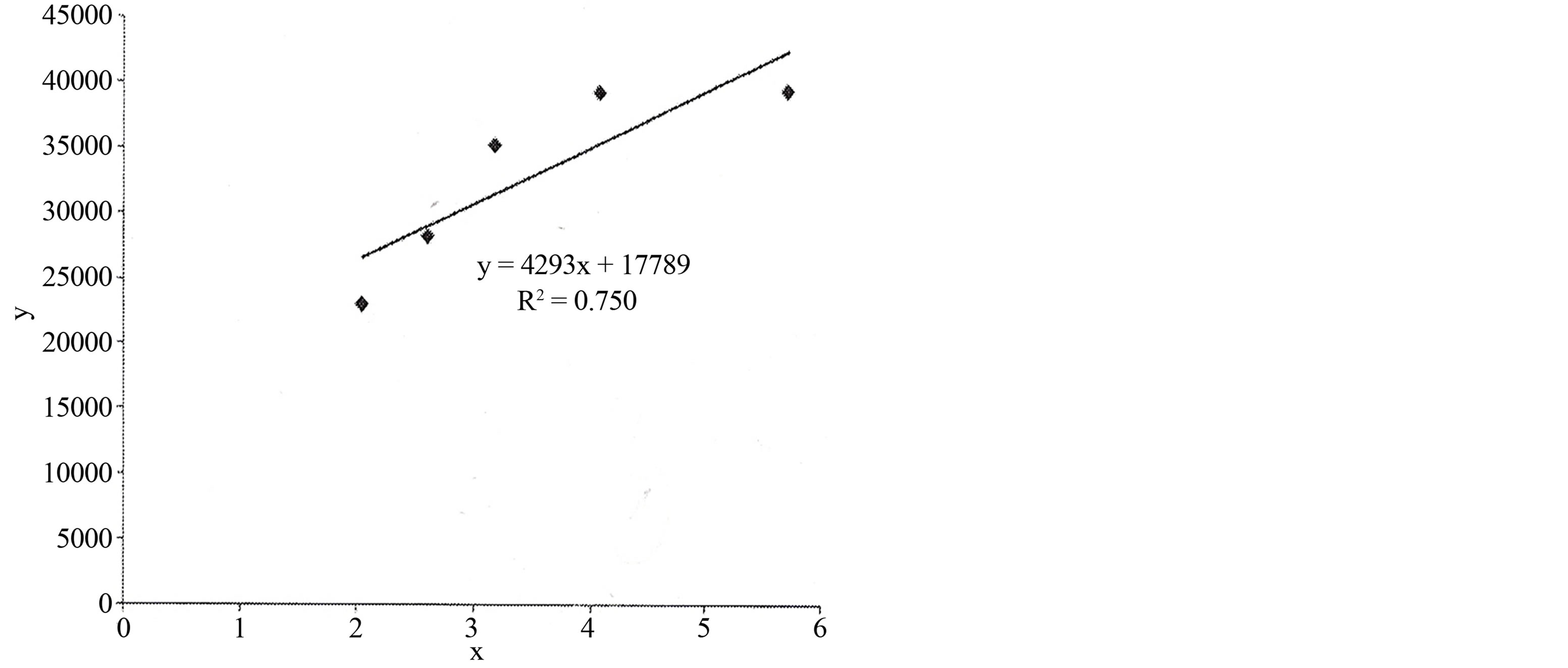
Figure 1. Dependence of tomato yield on standing density (linear approach; the initial coordinate as free “experimental point is not considered in the calculation scheme; у = М (ρ)—crop yield, х = ρ—scalar standing density); (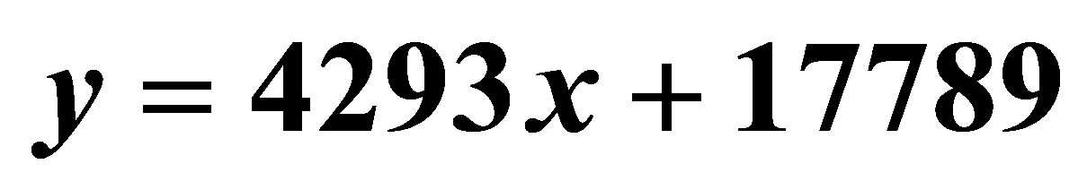 ;
; ).
).
points. In this case, the following expression are received
 (8)
(8)
(set of 5 “experimental” points).
 (9)
(9)

Figure 2. Dependence of tomato yield on standing density (quadratic approach, the initial coordinate as free “experimental point is not considered in the calculation scheme; у = М (ρ)—crop yield, х = ρ—scalar standing density as point is not considered in the calculation scheme);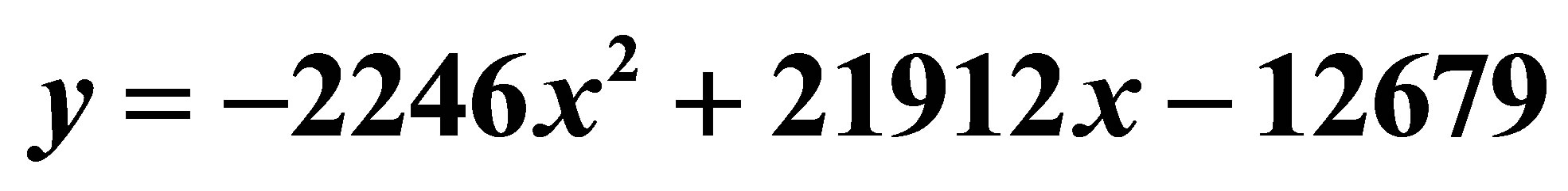 ;
; .
.
(set of 5 “experimental points + point of initial coordinate).
Connection of point of initial coordinate to the “experimental” points does not give significant changes in optimal approximation of calculation to the experimental data (the initial coordinate point as a free point can be
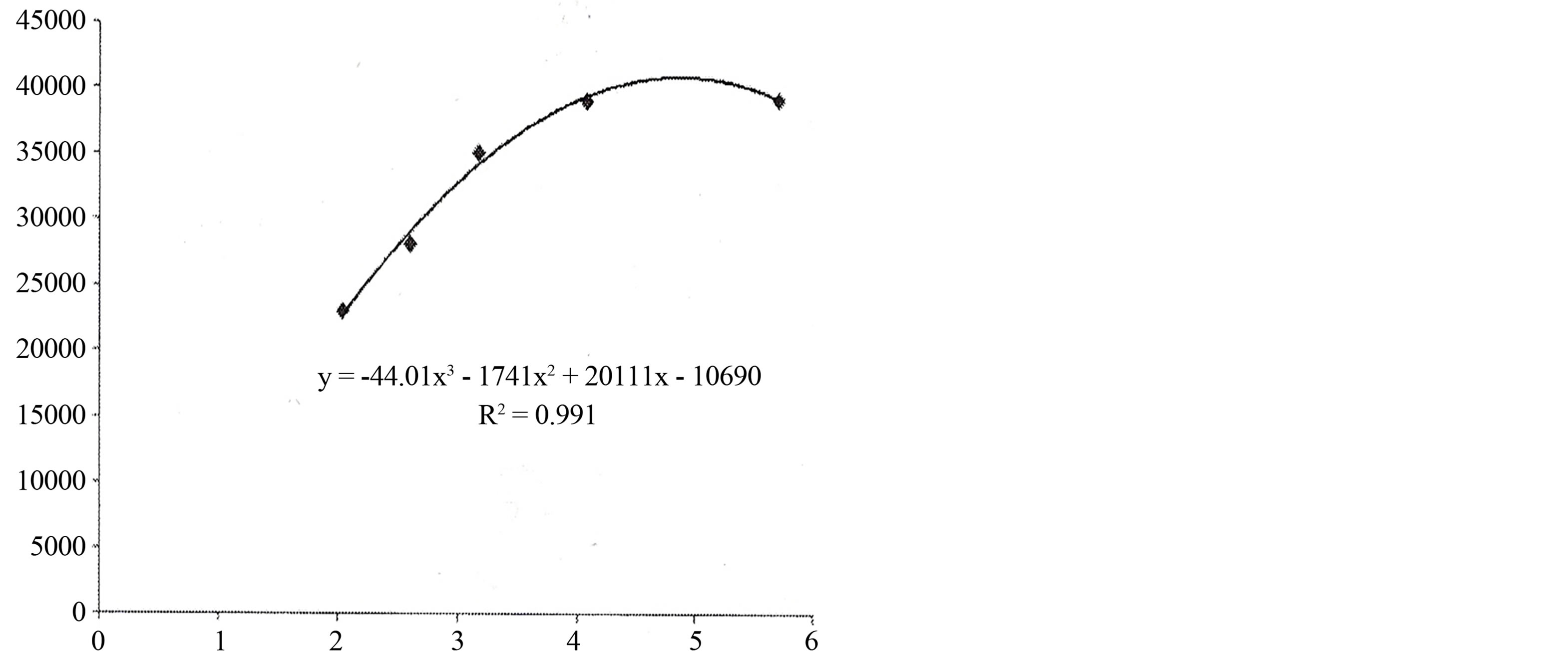
Figure 3. Dependence of tomato yield on standing density (cubic approach; The initial coordinate as free “experimental point is not considered in the calculation scheme; у = М (ρ)—crop yield, х = ρ—scalar standing density as point is not considered in the calculation scheme);  ;
; .
.
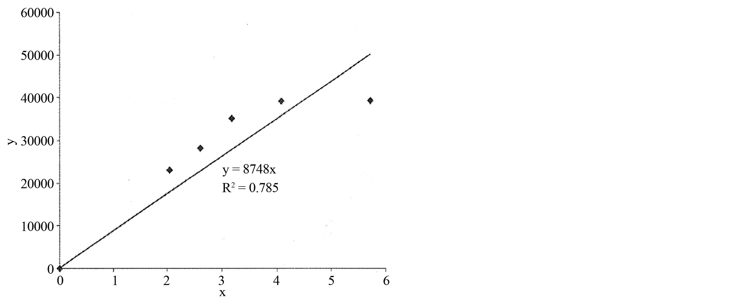
Figure 4. Dependence of tomato yield on standing density (linear approach; the initial coordinate is considered in the calculation scheme); ;
; .
.
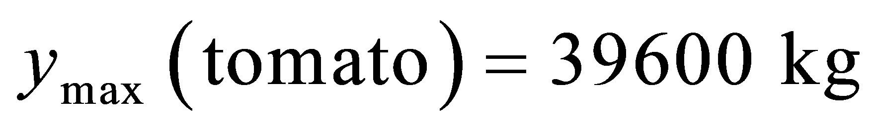
automatically connected to the “experimental” points on the plane {M, ρ}, as when there is no plant—ρ = 0; then the yield also is automatically equated to zero—M = 0). It means that the calculated scheme is steady even at very low values of the degree of freedom ν (ν = number of experimental points). A maximum value depending on productivity density for the tomato and pepper plants has been calculated and taken an average mark by means of quadratic and cubic approach functions for both versions (I version—a coordination introductory includes in calculation system; a consequence of the calculation was as the following:

Figure 5. Dependence of tomato yield on standing density (quadratic approach; the initial coordinate is considered in the calculation scheme);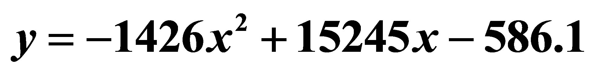 ;
; .
.
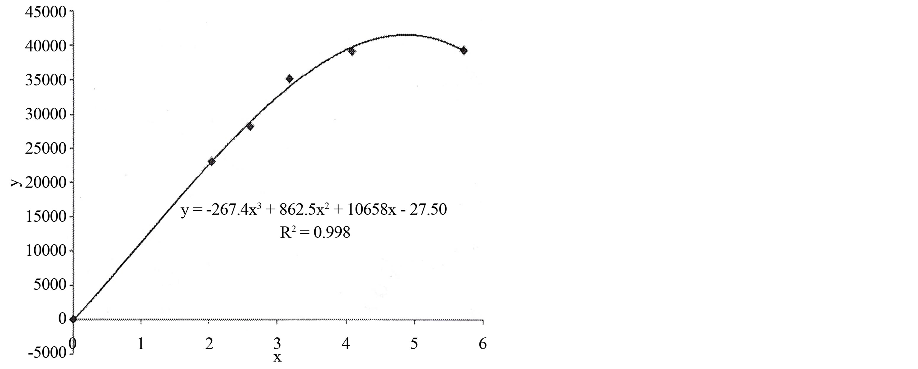
Figure 6. Dependence of tomato yield on standing density (cubic approach; the initial coordinate is considered in the calculation scheme);  ;
; .
.
 in
in .
.
 in
in .
.
3. Results and Their Discussion
3.1. Dependence of the Yield on Standing Density
In order to analyze the obtained data, first we will see the mechanisms of assimilation of nutrients through the root system.
Nutritious elements are developed through root system of the plant in three ways—interception, mass stream and diffusion. Barber and other [15] terms intercept by roots for the description of those soil nutritious elements that is on the root surface of the quantity of nutritious elements entering the plant through the root interception was assumed to be equal to their quantity in volume of soil corresponding to volume of root. For one-year crops the volume of roots in soil layer of 0 - 20 cm is usually less than 1% of soil volume. Hence due to the interception by roots less than 1% of available nutritious elements in the soil enter in the plant.
Mass flow rate—is the movement of nutrients through the soil to the roots in the convective flow of water, knitted water absorption by the plant. The quantity of nutritious elements moving in mass stream depends on absorption of water and concentration of these elements in it. This movement occurs on a distance exceeding distance defined by diffusion and quantities of nutritious elements arriving in 1 cm2 surface of the root due to the mass flow can be calculated by multiplying the water absorption rate (from 2 to 5 × 10⁻⁶ cm/sec) at concentration of these elements in equilibrium soil solution. Concentration of nutrients in soil solution of different soils also varies widely. In Table 2 it is given the concentration range of nutrients in soil solutions [16].
When interception by roots and mass stream does not provide supply of roots with enough quantity of the separate nutritious elements, the proceeding absorption reduces the concentration of available nutritious elements in soil at root surface. It leads to emergence of concentration gradient directed perpendicularly in relation to root surface that causes the subsequent diffusion of nutritious elements on a gradient to the root surface. Usually the distance for diffusive motion of nutritious elements in soil ranges from 0.1 to 15 mm. Consequently the contribution in root supply by nutritious elements by diffusion is made only by those which are in this zone of the soil.
From the above mentioned it can be concluded that the change in the distance between plants will not affect the mechanisms of development of nutrients through interception and diffusion. However the mechanism of the

Table 2. Nutritious elements.
mass flow is directly related to a standing density ρ. That is the less the distance between plants the more competition for the convective flow of water generated through the process of watering. On the other hand it is necessary to take into account the role of photosynthetic reaction in the process of growth and development of nutrients. The smaller distance between plants the more competition for solar reaction. It must be remembered that the smaller the average distance between plants, the larger number of plants more yield. That is, there is a certain point of “mathematical” experiment by which is balanced the factors outlined above. At approximation of the obtained data (dependence of tomato yield on scalar standing density in cubic approach was succeeded to find out above mentioned experimental point (in this case the maximum one). Maximum point corresponds to the value ρ which equals to 4.8 1/M2.
3.2. Dependence of Yield on Diet
Quantity of nitrogen in the composition of mineral fertilizer plays an important role in the growth process. But, excess quantities that are “surplus” may adversely affect the growth process and ecological indexes of soil. For “limiting” the excess amount of nitrogen we will turn to the method of inverse polynomial.
Inverse polynomials are usually modified so that it was possible to reflect the negative consequences associated with excess nitrogen. A typical value is
 (10)
(10)
where Y—yield, α—coefficient, taking into account the reduction in yield from excess nitrogen in soil А, BN, BP, BK—constants, N, P, K—application rates of nitrogen, phosphorus and potassium.
For evaluation of the reaction to nitrogen it is accepted:
For evaluation of the reaction to phosphorus it is accepted:
The maximum response to nitrogen is determined with the help of the following expression
Где  (11)
(11)
For limiting the excess nitrogen (minimum amount of nitrogen keep the value of the yield at the maximum point) it was chosen “experimental method”. It is based on the stepwise reduction of the amount of nitrogen on the scheme.
 (12)
(12)
In this case, at N90 the maximum value of the yield (for tomato) hardly changed, and the value of ρ corresponding to the maximum value of the yield shifted from 4.8 1/M2 to 5.1 1/M2. It should be noted that in this case the yield increase occurred due to a decrease in the cost of the agricultural measures.
4. Conclusions
1) For vegetable crops like tomato, eggplant and pepper it was found the value of scalar standing density corresponding to the maximum of the yield by approximation of the experimental data in cubic approach. In this case the supply circuit is selected in an optimum mode by means of mineral fertilizer N120P120K90. Such dependence is explained by the fact that the volume of their “own” soil plant is maximal close to each other. Further convergence creates “competition” for the development of moisture and solar radiation, and thus the yield falls.
2) Weak variation of the nitrogen content in the direction of decrease showed that there is a “stock” for increasing the “effective” yield due to decrease in the cost of mineral fertilizer. So with stepwise decrease in the amount of nitrogen it is revealed on scheme N120P120K90 → N100P120K90 → N90P120K90 that the maximum yield at N90 has hardly changed and the value of ρ corresponding to the maximum or shifted from 4.8 1/M2 to 5.1 1/M2.
Acknowledgements
This work has been executed in Institute of Soil Science and Agrochemistry of the National Academy of Sciences of Azerbaijan and was supported by the Science Development Foundation under the President of the Republic of Azerbaijan—Grant No. EİF-2010-1(1)-40/20-M-26.
REFERENCES
- R. W. Willey and S. B. Heath, “Plant Population and Crop Yield,” Advances in Agronomy, Vol. 21, 1969, pp. 281-321. http://dx.doi.org/10.1016/S0065-2113(08)60100-5
- J. H. M. Thornley, “Crop Yield and Planting Density,” Annals of Botany, Vol. 52, No. 2, 1983, pp. 257-259.
- G. Berry, “A Matematical Model Relating Plant Yield with Arrangement for Regularly Spaced Crops,” Biometrics, Vol. 23, No. 3, 1967, pp. 505-515. http://dx.doi.org/10.2307/2528011
- W. A. R. Lib, “Competition along a Nutriet Gradient,” Ecological Research, Vol. 15, No. 3, 2000, pp. 293-306.
- S. J. Shirtliffe and A. M. Johnston, “Yield-Density Relationships and Optimum Plant Populations in Two Cultivars of Solid-Seeded Dry Bean (Phaseolus vulgaris L.) Grown in Saskatchewan,” Canadian Journal of Plant Science, Vol. 82, No. 3, 2002, pp. 521-529. http://dx.doi.org/10.4141/P01-156
- L. G. Firbank and A. R. Watkinson, “On the Analysis of Competition within Two-Species Mixtures of Plants,” Journal of Applied Ecology, Vol. 22, 1985, pp. 503-517. http://dx.doi.org/10.2307/2403181
- R. H. Ellis, M. Sabahi and S. A. Jones, “Yield-Density Equations Can Be Extended to Quantify the Effect of Applied Nitrogen and Cultivar on Wheat Grain Yield,” Annals of Applied Biology, Vol. 134, No. 3, 1999, pp. 347- 352. http://dx.doi.org/10.1111/j.1744-7348.1999.tb05275.x
- D. J. Greenwood, T. J. Cleaner and M. K. Tuner, “Fertiliser Reguirements of Vegetable Crops,” Proceedings of Fertilizer Society, No. 145, 1974.
- J. H. M. Thornley, “Crop Response to Fertilizer,” Annals of Botany, Vol. 42, No. 4, 1978, pp. 817-826.
- Orudzheva, M. P. Babayev and S. M. Isgandarov, “Investigation of the Relations between Plant Density and Productivity, Poland, Nauka I Studia,” Nauk Biologicz Nych, Medycyna, Weterynaria, Vol. 22, No. 67, 2012, pp. 46- 53.
- Orudzheva, M. P. Babayev, S. M. Isgandarov and A. Alizade, “Influence of the Plant Density on Productivity,” Soil-Water Journal, Vol. 2, No. 2, 2013, pp. 1021-1028.
- Orudzheva, “Change of the Microorganisms Quantity in Irrigative Gleyey-Yellow under Vegetable Soils,” American Journal of Plant Sciences, Vol. 3, No. 12, 2012, pp. 1746-1751.
- M. P. Babayev and N. İ. Oudzheva, “Assessment of the Biological Activity of Soils in the Subtropical Zone of Azerbaijan,” Eurasian Soil Science, Vol. 42, No. 10, 2009, pp. 1163-1169. http://dx.doi.org/10.1134/S1064229309100111
- Orudzheva, “Microbiological Characteristcs of Different Types of Irrigated Soils in the Subtropical Zone of Azerbaijan,” Eurasian Soil Science, Vol. 44, No. 11, 2011, pp. 1241-1249. http://dx.doi.org/10.1134/S1064229311030094
- S. A. Barber, J. M. Walker and E. H. Vasey, “Mechanisms for the Movement of Plant Nutrients from the Soil and Fertibzer to the Plant Root,” Journal of Agricultural and Food Chemistry, Vol. 11, No. 3, 1963, pp. 204-207. http://dx.doi.org/10.1021/jf60127a017
- S. A. Barber, “Nutrients in the Soil and Their Flow to Plant Roots,” Range Sci, Series No. 2b, Colorado State University Fort Collins, 1974, pp. 161-168.
NOTES
*Corresponding author.