Open Journal of Air Pollution
Vol.2 No.1(2013), Article ID:29010,12 pages DOI:10.4236/ojap.2013.21002
Organic and Elemental Carbon in Atmospheric Fine Particulate Matter in an Animal Agriculture Intensive Area in North Carolina: Estimation of Secondary Organic Carbon Concentrations
1Department of Animal Science, Michigan State University, East Lansing, USA
2Department of Biological and Agricultural Engineering, North Carolina State University, Raleigh, USA
3RTI International, Research Triangle Park, USA
Email: qfli@msu.edu, *lwang5@ncsu.edu, rkmj@rti.org, sbshah3@ncsu.edu
Received December 11, 2012; revised January 17, 2013; accepted January 27, 2013
Keywords: Secondary Organic Carbon (SOC); Organic Carbon (OC); Elemental Carbon (EC); PM2.5; Agriculture Area
ABSTRACT
Carbonaceous components contribute significant fraction of fine particulate matter (PM2.5). Study of organic carbon (OC) and elemental carbon (EC) in PM2.5 may lead to better understanding of secondary organic carbon (SOC) formation. This year-long (December 2008 to December 2009) field study was conducted in an animal agriculture intensive area in North Carolina of United States. Samples of PM2.5 were collected from five stations located in an egg production facility and its vicinities. Concentrations of OC/EC and thermograms were obtained using a thermal-optical carbon analyzer. Average levels of OC in the egg production house and at ambient stations were 42.7 µg/m3 and 3.26 - 3.47 µg/m3, respectively. Average levels of EC in the house and at ambient stations were 1.14 µg/m3 and 0.36 - 0.42 µg/m3, respectively. The OC to total carbon (TC) ratios at ambient stations exceeded 0.67, indicating a significant fraction of SOC presented in PM2.5. Principal factor analysis results suggested that possible major source of in-house PM2.5 was from poultry feed and possible major sources of ambient PM2.5 was from contributions of secondary inorganic and organic PM. Using the OC/EC primary ratio analysis method, ambient stations SOC fractions ranged from 68% to 87%. These findings suggested that SOC could appreciably contribute to total PM2.5 mass concentrations in this agriculture intensive area.
1. Introduction
Particulate matter (PM) contains a significant fraction of carbonaceous materials. The carbonaceous materials are usually classified as elemental carbon (EC) and organic carbon (OC) [1]. Elemental carbon generates predominantly from incomplete combustion process, and it has been used as a tracer for primary OC (POC) [2]. Organic carbon includes POC, which refers to carbon material emitted in particulate form, and secondary OC (SOC), which is formed through atmosphere physical and chemical reactions [1]. Carbon-containing components (EC and OC) occupy very important fractions of PM, and they account typically 10% to 50% of atmospheric PM mass [1,3]. Although knowledge about POC and SOC is important to develop strategies for controlling particulate carbon pollution, quantification has been difficult to accomplish because of the complexity and no simple analytical methods available. Several methods have been applied to estimate the fraction of SOC [2,4-9]. The thermographic analysis method, which is performed on PM samples collected on quartz filters, can classify organic compounds into groups [7,8]. In this method, a carbon thermogram may be constructed by plotting the evolved carbon as a function of temperature. The thermogram peaks can then be used for source allocation, i.e., primary and secondary portions of carbon-containing component studies [5,8]. Hildemann, et al. [6] used carbon isotopic composition (14C/12C) to estimate the SOC in the Los Angeles basin. Turpin, et al. [2,9] applied OC/EC ratios to quantify the presence of SOC. Castro, et al. [4] estimated SOC using the minimum ratio of OC/ EC. The OC/EC primary ratio analysis is an acceptable method for SOC estimation.
In the United States (US) the Clean Air Act (CAA) was signed into law in 1970 and the US environmental protection agency (EPA) established the national ambient air quality standards (NAAQS) to protect public health and environment under the CAA. To assess national ambient air quality and implement NAAQS, the EPA has established a comprehensive ambient air monitoring program, which has been carried out by state and local agencies [11]. All the EPA monitoring networks have provided numerous high quality datasets for air quality and public health studies. However, these existing networks do not provide enough representative scientific data for assessment of ambient air quality in rural areas, especially in agricultural intensive areas.
As of the most recent Agricultural Census [12], North Carolina (NC) ranked second in the nation in the production of hog and poultry. Because of the rapid growth of swine and poultry industry, significant increases of ambient air pollutant concentrations (e.g. NH3) were observed in NC coastal plain regions [13,14]. Regional intensive agricultural activities (especially livestock and poultry industry) pose substantial risks to air quality and public health. Quantitative information concerning the presence of SOC is still scarce, and to the authors’ knowledge, there is no publication addressing this subject quantitatively in animal agriculture intensive areas.
In this study, a field investigation was conducted to characterize the OC and EC of PM2.5 inside and in the immediate vicinity of a large commercial egg production farm. The objectives were to: 1) provide an OC/EC dataset for animal agriculture intensive areas; 2) present OC thermal characterization information; 3) assess POC and SOC in order to understand the contribution of SOC to the total organic carbon (TOC) in PM2.5.
2. Methodology
2.1. The Research Site and Field Sampling Locations
The field sampling of PM2.5 was conducted in an animal agriculture intensive area in NC. As shown in Figure 1, samples of PM2.5 were simultaneously taken at five stations: an emission source (a high rise egg production house: ST1), and the ambient stations (ST2-5) surrounding the farm nearby the property lines of the egg production farm. The filed sampling campaign covered four seasons from December 2008-December 2009 and 312 samples were taken. While the data series were not continuous, the numbers of samples were sufficient to give a very good representation of the variability of the concentrations over the sampling periods.
Sampling was performed with Partisol (Model 2300) chemical speciation samplers, operated for durations ranging from 8 to 24 hours. Three cartridges with different filters (Nylon, Teflon and Quartz) were used to collect PM2.5 samples. Nylon filter was used for ion analyses [15,16], Teflon filter was used for trace element and mass analyses [17], and Quartz filter was used for organic and element carbon analyses. Each cartridge contains a sharp-cut PM2.5 impactor operating at a flow rate of 10.0 L/min (nylon and quartz) or 16.7 L/min (Teflon). Filters were kept and transported to field in individual petri dishes. After sampling, exposed filters were stored at 4˚C and transported to the analysis laboratory.
2.2. Thermal-Optical Aerosol Analyzer: Carbon Analyses
The collected quartz filters were analyzed for OC/EC at RTI aerosol laboratory (RTP, NC, US) using a ThermalOptical Carbon Aerosol Analyzer (Sunset Laboratory Inc., OR, USA). Figure 2 shows the schematic diagram of the analyzer. A punch of subsample from a quartz filter was placed in a quartz boat of the analyzer and the light diode laser was used to monitor transmittance of the filter during analysis. A thermocouple was, used to monitor sample temperature during analysis. The front oven

Figure 1. The layer farm layout and the PM2.5 sampling stations [10].
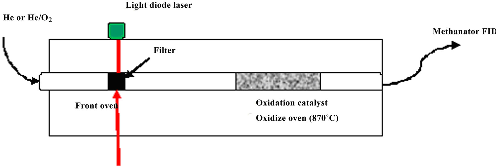
Figure 2. Schematic diagram of a thermal-optical carbon analyzer.
heating program was the NIOSH-like method used as part of the PM2.5 Speciation Trends Network [18]. The NIOSH method started with a 10-sec purge, followed by four 60-sec temperature ramps (310˚C, 480˚C, 615˚C and 900˚C) in a non-oxidizing atmosphere (Helium), then after cooling oven to 600˚C, a series of 45-sec four heating ramps (600˚C, 675˚C, 750˚C, 825˚C) and 120-sec at 920˚C was applied in a 2% oxygen in helium atmosphere (Figure 3). All carbon species evolved from the filter are converted to carbon dioxide (CO2) in oxidizer oven (870˚C), and CO2 is reduced to methane and detected using a flame ionization detector (FID). OC Pk1, OC Pk2, OC Pk3 and OC Pk4 were the integration of the FID signal under four 60-sec temperature ramps in Helium atmosphere (Figure 3). Total OC is the summation of OC Pk1, OC Pk2, OC Pk2, OC Pk4 and pyrolysed OC. Peaks integrated at 2% O2/98% He atmosphere and subtracted pyrolysed OC were EC. The optical measurement was used to correct for pyrolysis or charring of OC during heating process. This method reports only carbon contents and does not directly account for the mass of hydrogen, oxygen and any other elements.
2.3. Estimations of SOC Concentrations Using the Minimum Value of OC/EC Ratio Method
At this research site, there were evidences of the influence of SOC that were transported or formed in this agriculture intensive sampling area. Since no experimenttal method could be used to directly measure SOC fraction, Turpin and Huntzicker [2] proposed using EC and OC data to estimate the SOC fraction. Elemental carbon, emitted mainly by combustion sources, was used as a tracer of primary fraction of OC. In the proposed method, for a given site, the OC-to-EC ratio ((OC/EC)pri), representative of the primary emissions of EC and OC, was assumed to be relative constant and do not evolve significantly.
The concentration of SOC can then be calculated from the equation:
 (1)
(1)
where, OCtotal is the total OC, the summation of OC Pk1, OC Pk2, OC Pk2, OC Pk4 and pyrolysed OC.
Statistical analyses were performed using SAS/STAT software, version 9.2 (SAS Institute Inc., Cary, NC, USA). The paired t-test analyses were performed to test the statistical differences between different stations. Multivariate analyses were conducted to elucidate possible relationship among them. A factor analysis was conducted for the correlation matrix of the variable analyzed, using principle component analysis as the extraction methods. The rotation method of VARIMAX was used. Variable standardization was performed in order to have means of zeros and variances of one.
3. Results and Discussion
3.1. Overall Means of Samples from In-House and Ambient Stations
The overall mean concentrations of PM2.5 mass, OC, EC, and total carbon (TC, the summation of OC and EC) are given in Table 1, which also includes the numbers of samples, standard deviations (Std.), medians, minimums and maximums. In poultry house (ST1), the average OC and EC concentrations were higher than ambient stations. The high OC concentrations at ST1 indicated that most of PM2.5 was contributed by organic matter (e.g., crude feed protein, crude feed fiber, and animal dander) generated from mechanical processes. In the poultry house, there was no bio-based fuel heating system, so there was very little EC generated in the poultry houses. The reported EC at ST1 might be due to the uncertainty from the pyrolysis correction [29]. At ambient stations (ST2-5), OC concentrations were slightly higher than 3.0 µg/m³, and EC concentrations were about 10% of OC. The average OC and EC levels for ambient stations were within the range given by other studies at other regional rural or background sites (Table 2). The OC to PM2.5 mass ratios (36% - 40%) were higher than most values reported in the literature. The possible reasons may be due to the
 (a)
(a)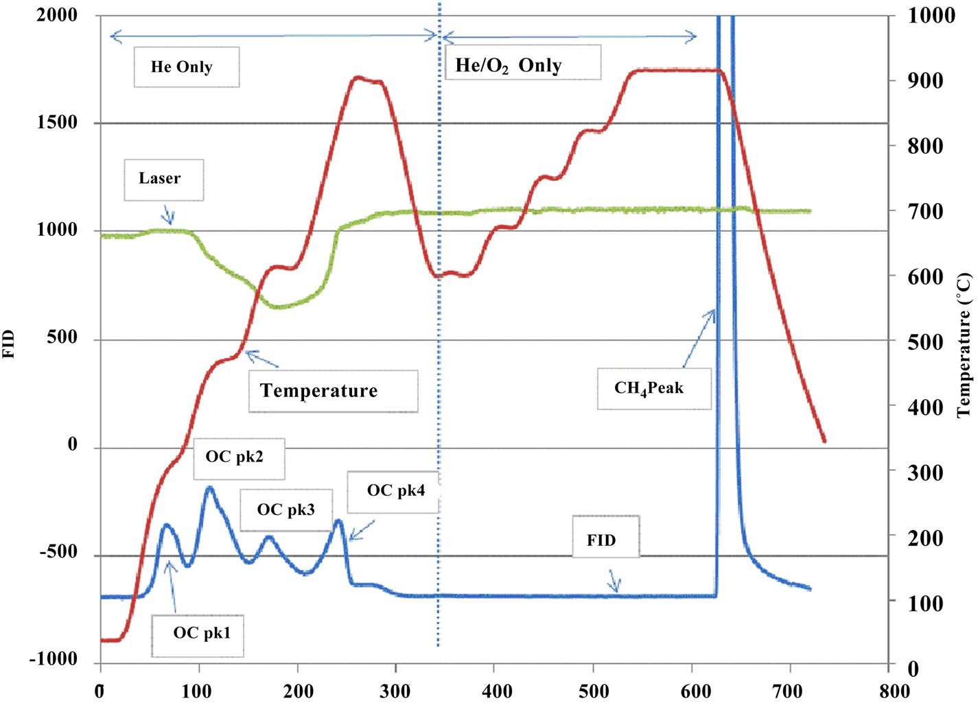 (b)
(b)
Figure 3. Typical thermograms. (a) a sample from the in house station; (b) a sample from an ambient station.
fact that this research site was in a rural agriculture area with a large egg production facility. Local agriculture activities might result in different OC to PM2.5 ratios from other areas if the farming practices are different. Turpin and Huntzicker [9] and Chow, Watson [20] used the ratios of OC to TC concentrations to study emission and transformation characteristics of carbonaceous species in particulate. As it is well known, EC originates primarily from direct emissions, whereas OC can originnate from direct emissions and atmospheric transformations. The average ratios of OC/TC were similar at four ambient stations (Table 1), and these ratios were higher than the reported values [20]. The distribution of OC/TC ratios from all ambient sites is shown in Figure 4. The OC/TC ratio were greater than most of the OC/TC ratio of the primary aerosol (emissions by different sources), which indicated secondary formation occurred [2,21]. The high OC/TC ratios at the ambient stations were pos-
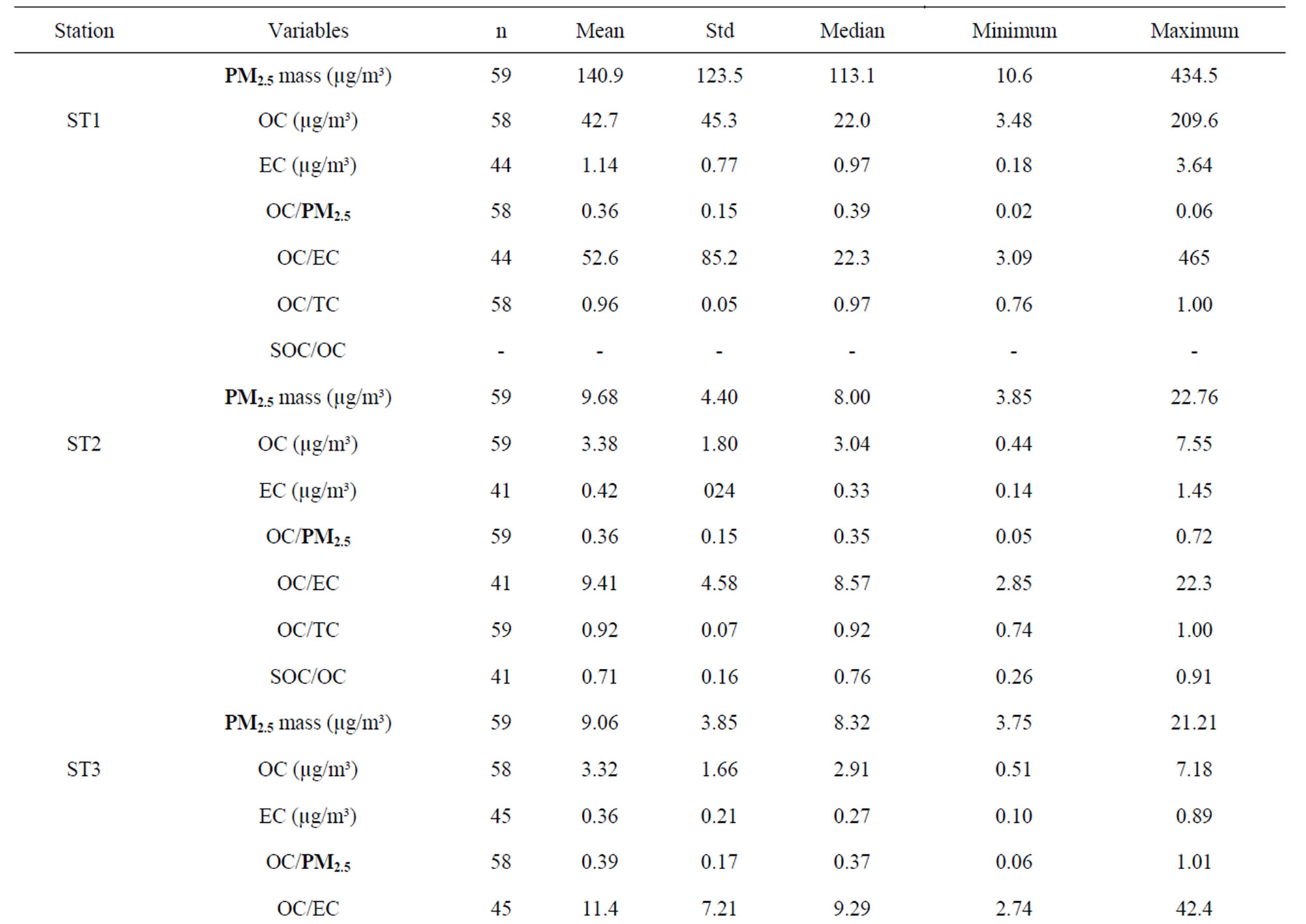

Table 1. Descriptive statistics of mass concentration, OC, and EC of PM2.5 samples.

Table 2. Elemental and organic carbon levels found in PM2.5 from different regions of the world.
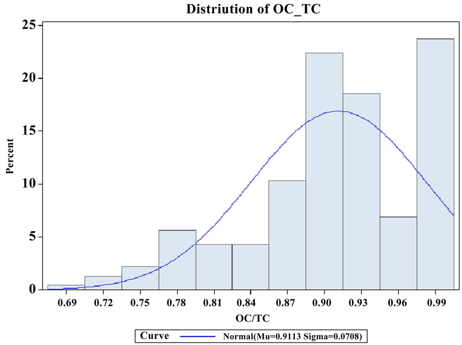
Figure 4. The distribution of OC/TC ratios at ambient stations.
sible due to biogenic emissions, anthropogenic emissions, and atmospheric transport and transformation. Forest fire, natural gas home appliances, meat charbroiling, etc. might also result in high OC/TC ratio [21].
By checking into the relationship between OC and EC, the relative importance of biogenic and anthropogenic emissions of OC and transport can be examined [22]. If there was strong correlation between OC and EC, it was likely that they were transported simultaneously from other regions or emitted from a similar source.
The relationships between OC and EC concentrations at ambient stations (ST2-5) are shown in Figure 5. The observed weak relationships between OC and EC (correlation coefficients r < 0.1) suggested that OC and EC of PM2.5 at this research site were not transported simultaneously from other regions, and the local biogenic and anthropogenic OC emissions were very important.
3.2. Thermograms
Figure 3 illustrates the distinctions between samples collected in house and at ambient stations. The marked peaks of OC Pk1, OC Pk2, OC Pk3, OC Pk4, pyrolysed OC and EC are the principal features of the thermograms. The OC Pk1 observed approximately 310˚C corresponds to the volatilization of lower molecular weight organics. The OC Pk2, OC Pk3, and OC Pk4 at approxi-

Figure 5. Relationship between OC and EC concentrations at ambient stations.
mately 480˚C, 615˚C and 950˚C correspond to volatilizetion and decomposition of higher molecular weight species. Pyrolysed OC was detected in the O2/He atmosphere at 600˚C prior to the return of transmittance to its original value.
As shown in Figure 3, the thermograms from source and receptor stations were significantly different. The thermogram results are summarized in Table 3, where all results were normalized to TC to check for consistency among samples from different stations. It was clear that all ambient stations had very similar thermogram results with a pronounced high volatile peak (OC Pk1) as compared to those of the source samples (ST1). Organic carbon in the intermediate range of volatility (OC Pk2) comprised 47% of the carbon mass for the source PM2.5 samples, which was significantly higher than that of ambient stations. The ambient seasonal variations of OC fractions are shown in Figure 6. The relatively high volatile carbon fraction (OC Pk1) might attribute to direct biogenic and anthropogenic emissions. Since partitioning of the high volatile OC (Pk1) between gas and particle phases were temperature dependent [23], the cold seasons had higher OC Pk1 fraction than warm sea sons. The OC in the intermediate range of volatility (OC Pk2 and Pk3) might attribute from secondary processes. The positive temperature dependence might be related to changes in
 (a)
(a)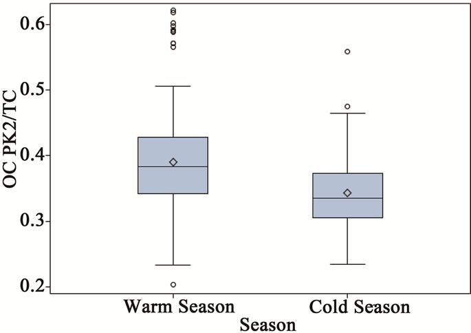 (b)
(b)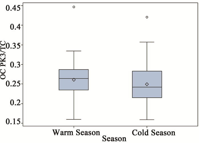 (c)
(c)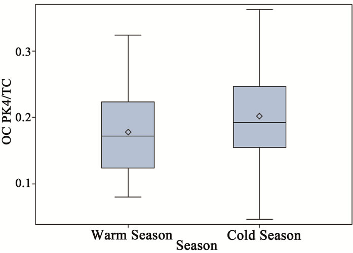 (d)
(d)
Figure 6. Seasonal variations of OC fractions for ambient PM2.5 samples (a = OC Pk1/TC, b = OC Pk2/TC, c = OC Pk3/TC and d = OC Pk4/TC).
the chemical mechanism and increased secondary chemical reaction rate at warm seasons (Figure 6) [1]. The low volatility fraction (OC Pk4) presented in ambient samples in cold seasons was significantly higher than that in warm seasons, and it might attribute from primary emissions.
3.3. Source Apportionment by Principal Factor Analyses
The principal factor analysis was performed on OC, EC, and major ion data for source apportionment. Samples of PM2.5 collected on Nylon filters were analyzed for six major ions using Ion Chromatography (IC). Analysis of the ion concentration data has been reported elsewhere [15,16]. In this study, , Na+,
  , Cl− and
  were included in the source apportionment analyses. In the process of principal factor analysis, a scree plot was applied to visually determine how many components to retain (Figure 7). An elbow occurred in the plot in Figure 7 at about I = 4. In this case, it appears that four (or perhaps three) principal components effectively summarized the total sample variance. Factor loadings of variables analyzed for the four components extracted from ST1 and ST2-5 are shown in Table 4. These four components accounted for 84% and 81% of total variance in house and at ambient stations, respectively. The first factor (Pc 1) at ST1, explaining 43% of the variance, had high correlation coefficients (factor loading) for OC Pk2, OC Pk3 and OC Pk4, indicating possible source from poultry feed (e.g., crude protein, crude fiber) and/or animal dander. The second factor (Pc 2) at ST1, explaining 15% of the variance, had high factor loading for Cl− and Na+, indicating possible source from poultry feed salt additives [15]. The third and fourth factors represent OC Pk1 (relatively high volatile OC) and
 . The possible sources of OC Pk1 and
  might be from manure due to bacteria biological processes and the formation of volatile organic and inorganic compounds. At ambient stations (ST2-5),
  and
and  had high factor loading in the first factor, explaining 44% of the variance. This fraction of PM2.5 was due to the formation of secondary inorganic PM [15]. The second factor at ambient stations, explaining 14% of the variance, had high corre-
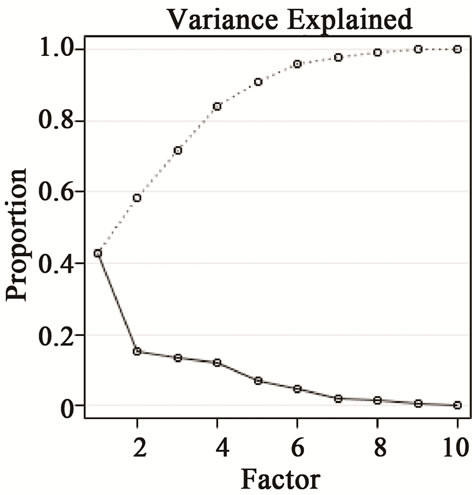
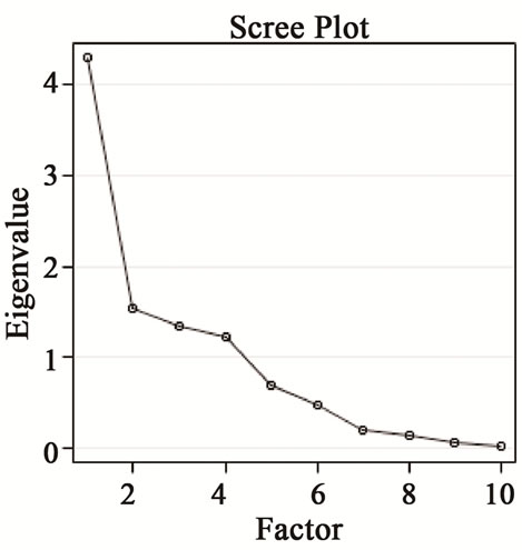

Figure 7. The scree plot and variance explained by factors using ions and OC/EC data at ST1.
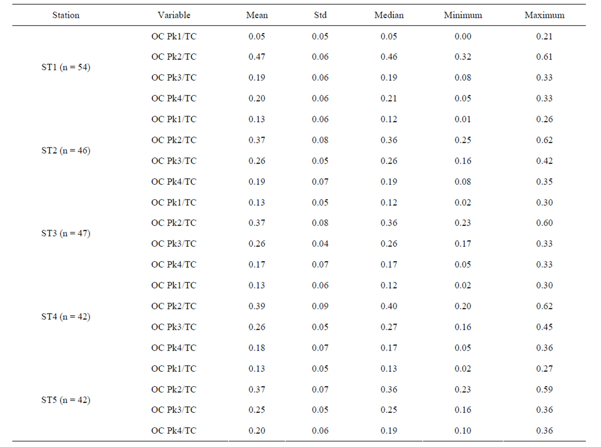
Table 3. Summary of thermal analyses for PM2.5 samples taken at ST1-ST5 in (µg/m3)/( µg/m3).
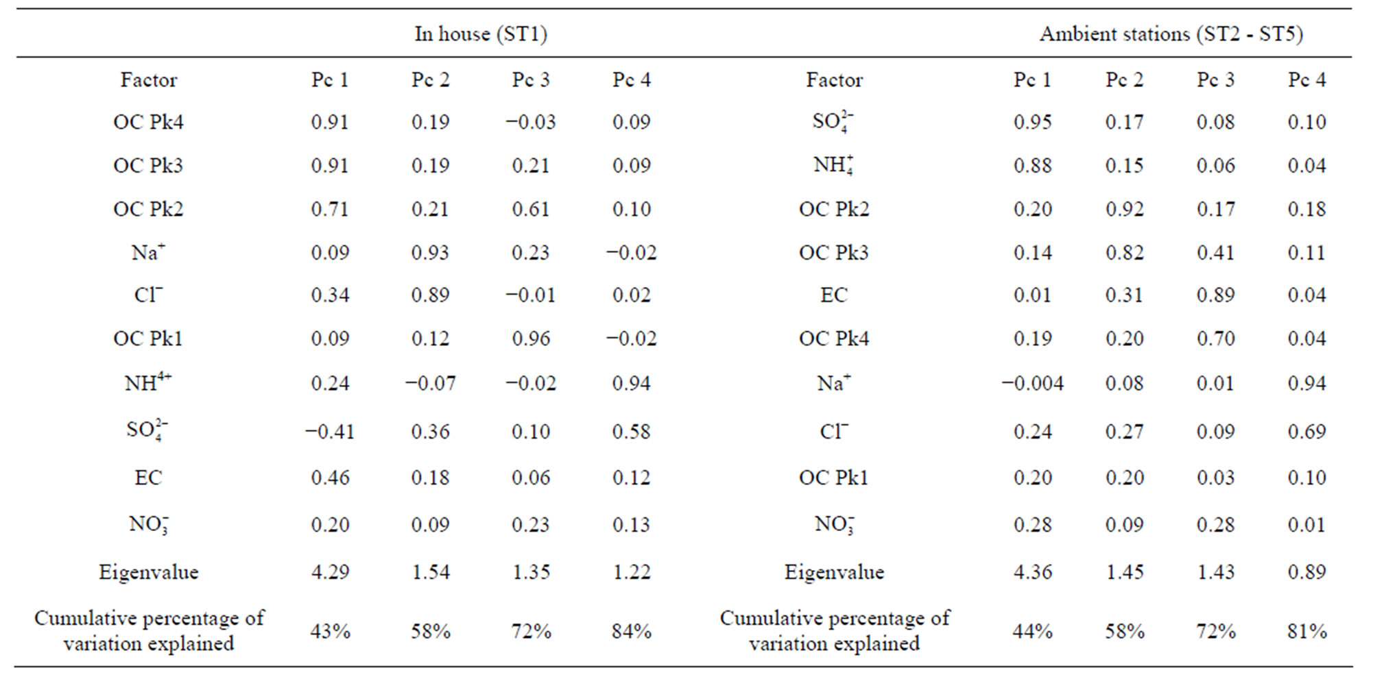
Table 4. Factor loadings of components extracted from ST1 (in house) and ST2-5 (ambient stations).
lation coefficients for OC Pk2 and OC Pk3, and might be attributed to the formation of secondary organic PM. The third factor at ambient stations, explaining 14% of the variance, had high factor loading for OC Pk4 and EC, indicating possible source from primary emissions (e.g. combustion process). The fourth factor at ambient stations, explaining 9% of variance, had high factor loading for Na+ and Cl−, indicating possible nearby poultry emission influence and marine source from Atlantic Ocean, which was about 240 km away.
3.4. Concentrations of SOC Concentrations Determined by the Minimum Value of OC/EC Ratio Method
In Equation (1), the (OC/EC)pri could be determined using several methods [2,4,9,24]. As shown in Figure 5, there was a clear minimum value of 2.1 for the OC/EC ratio. This (OC/EC)pri ratio of 2.1 was in the range generally presented in the literature [5,21]. The clear minimum OC/EC ratio indicated that the primary carbonaceous PM varied little in relative composition, so this minimum value of OC/EC ratio was used to calculate the SOC concentrations [5].
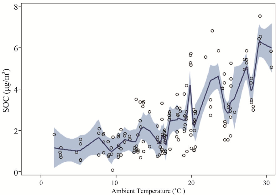
Presented in Table 1, the SOC were calculated using Equation (1) with the primary ratio of 2.1. Four ambient stations had similar SOC fractions, and they ranged from 68% to 87%, which were little higher than the reported values in literature [5,21]. At the ambient stations, SOC concentrations and fractions showed a clear increasing tendency with temperature (Figure 8). The increase in temperature correlated with the increase in SOC concentrations, which was contrary to some observations and modeling studies [25,26]. It is well known that there is greater formation of radicals (e.g., OH, NO3 and O3) in high temperature than that in low temperature, so SOC formation would be enhanced by higher temperature. However, higher temperature would reduce subsequent gas-to-particle phase partitioning, nucleation and condensation [1,21]. As a result, the relationship between SOC formation and temperature should be considered as integrated effects of radical formation, gas-to-particle phase partitioning, nucleation and condensation. The overall effect of temperature in this study appeared to be positive.
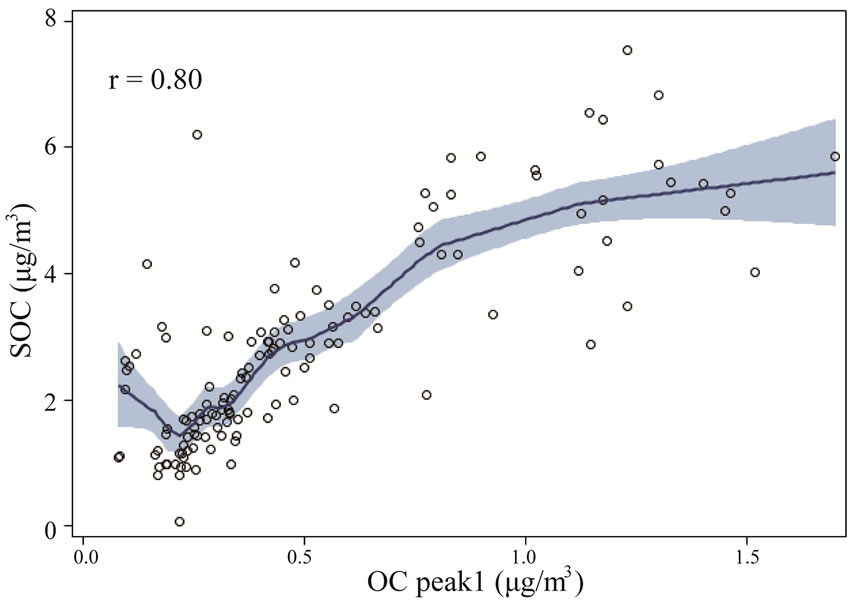
Figure 9 shows the relationship between thermogram peaks and SOC. Secondary organic carbon was highly correlated with OC Pk1, OC Pk2, and OC Pk3 (Figures 9(a)-(c)), and less correlated with OC Pk4 (Figure 9(d)), and not correlated with EC (Figure 9(e)). These results suggested that in the rural atmosphere the key factors determining SOC formation were VOC precursors (related to OC Pk1), and favorable meteorological conditions for gas-to-particle conversion, radical formation, nucleation and condensation. Organic carbon in higher
 (a)
(a) (b)
(b)
Figure 8. SOC concentrations a) and SOC fractions b) at ambient stations vs. temperature. The solid lines are locally weighted scatterplot smoothing, and the shaded areas are 95% confidence intervals.
molecular weight species (related with OC Pk4) and EC emitted during the incomplete combustion of fossil and biomass, which was mainly as submicron particles, had no major influence on SOC formation.
4. Conclusion
This study investigated the carbonaceous components of PM2.5 in an egg production facility and its vicinity. The high OC fraction in poultry house (36%) indicated that organic matters from feed made significant contribution to total PM2.5 mass. The ambient OC to PM2.5 mass ratios (36% - 40%) were higher than most reported values in the literature. The ambient OC/TC ratio exceeded 0.67, indicating a significant fraction of SOC in PM2.5. All four ambient stations had very similar thermogram results with a pronounced high volatile peak compared to the source samples. Principal factor analysis revealed that, in house, feed was one of major sources of OC; at ambient, he intermediate volatile OC might attribute from seconddary formation. The presence of a minimum OC/EC ratio of 2.1 indicated that the primary carbonaceous PM varied
 (a)
(a)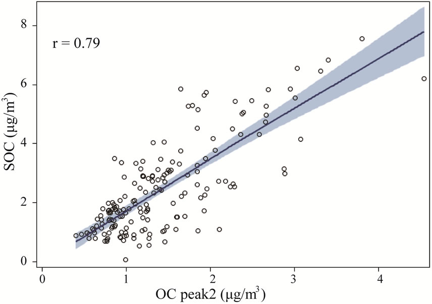 (b)
(b)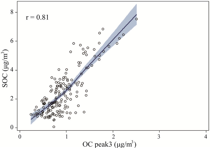 (c)
(c)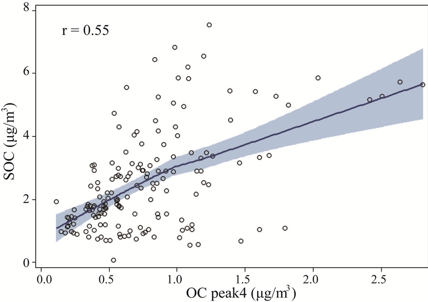 (d)
(d)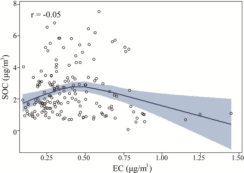 (e)
(e)
Figure 9. The relationships between thermogram peaks and SOC concentrations. The solid lines are locally weighted scatterplot smoothing, and the shaded areas are 95% confidence intervals. the “r” represents Pearson correlation coefficient.
little in relative composition. Four ambient stations had similar SOC fractions, ranged from 68% to 87%. The correlation between thermogram peaks and SOC suggested that in the rural atmosphere, the key factors determining SOC formation were VOC precursors, and favorable meteorological conditions for atmospheric physical and chemical reactions. Overall, the findings gained from this study, with additional consideration of different source emissions and meteorology information, will lead to better understanding of SOC formatin and its dynamics in the atmosphere.
5. Acknowledgements
This study was supported in part by the NSF-CAREER Award (No. CBET-0954673) and the National Research Initiative Competitive Grant No. 2008-35112-18757 from the USDA Cooperative State Research, Education, and Extension Service Air Quality Program. The authors acknowledge the generous support and collaboration of the egg producer. Help from Zifei Liu for the field PM2.5 sample collection is thankfully acknowledged.
REFERENCES
- J. H. Seinfeld and S. N. Pandis, “Atmospheric Chemistry and Physics: From Air Pollution to Climate Change,” 2nd Edition, John Wiley & Sons, Inc, New Jersey, 1998.
- B. J. Turpin and J. J. Huntzicker, “Secondary Formation of Organic Aerosol in the Los-Angeles Basin: A Descriptive Analysis of Organic and Elemental Carbon Concentrations,” Atmospheric Environment. Part A. General Topics, Vol. 25, No. 2, 1991, pp. 207-215. doi:10.1016/0960-1686(91)90291-E
- J. Schwarz, X. G. Chi, W. Maenhaut, M. Civis, J. Hovorka and J. Smolik, “Elemental and Organic Carbon in Atmospheric Aerosols at Downtown and Suburban Sites in Prague,” Atmospheric Research, Vol. 90, No. 2-4, 2008, pp. 287-302. doi:10.1016/j.atmosres.2008.05.006
- L. M. Castro, C. A. Pio, R. M. Harrison and D. J. T. Smith, “Carbonaceous Aerosol in Urban and Rural European Atmospheres: Estimation of Secondary Organic Carbon Concentrations,” Atmospheric Environment, Vol. 33, No. 17, 1999, pp. 2771-2781. doi:10.1016/S1352-2310(98)00331-8
- E. C. Ellis and T. Novakov, “Application of ThermalAnalysis to the Characterization of Organic Aerosol-Particles,” Science of the Total Environment, Vol. 23, 1982, pp. 227-238. doi:10.1016/0048-9697(82)90139-5
- L. M. Hildemann, D. B. Klinedinst, G. A. Klouda, L. A. Currie and G. R. Cass, “Sources of Urban Contemporary Carbon Aerosol,” Environmental Science & Technology, Vol. 28, No. 9, 1994, pp. 1565-1576.
- T. Novakov, “Particulate Carbon,” Plenum Press, New York, 1982. doi:10.1021/es00058a006
- J. R. Turner and S. V. Hering, “Vehicle Contribution to Ambient Carbonaceous Aerosols by Scaled Thermograms,” Aerosol Science and Technology, Vol. 12, No. 3, 1990, pp. 620-629. doi:10.1080/02786829008959376
- B. J. Turpin and J. J. Huntzicker, “Identification of Secondary Organic Aerosol Episodes and Quantitation of Primary and Secondary Organic Aerosol Concentrations during SCAQS,” Atmospheric Environment, Vol. 29, No. 23, 1995, pp. 3527-3544. doi:10.1016/1352-2310(94)00276-Q
- L. Wang-Li, Q.-F. Li, K. Wang, B. W. Bogan, J.-Q. Ni, E. L. Cortus and A. J. Heber, “National Air Emissions Monitoring Study—Southeast Layer Site: Part I-Site Specifics and Monitoring Methodology,” Transactions of the ASABE, 2013.
- Environmental Protection Agency, “The Ambient Air Monitoring Program,” 2012. http://epa.gov/airquality/qa/monprog.html.
- K. Krueger, “N.C. Agricultural Statistics,” 2011. http://www.ncagr.gov/stats/2011AgStat/AgStat2011.pdf.
- J. Walker, D. Nelson and V. P. Aneja, “Trends in Ammonium Concentration in Precipitation and Atmospheric Ammonia Emissions at a Coastal Plain Site in North Carolina, USA,” Environmental Science & Technology, Vol. 34, No. 17, 2000, pp. 3527-3534. doi:10.1021/es990921d
- V. P. Aneja, D. R. Nelson, P. A. Roelle, J. T. Walker and W. Battye, “Agricultural Ammonia Emissions and Ammonium Concentrations Associated with Aerosols and Precipitation in the Southeast United States,” Journal of Geophysical Research-Atmospheres, Vol. 108, No. D4, 2003. doi:10.1029/2002JD002271
- Q.-F. Li, L. Wang-Li, Z. Liu, J. Walker and R. K. M. Jayanty, “Major Ionic Components Characterizations of Fine Particulate Matter in an Animal Feeding Operation Facility and Its Vicinity,” Prepared for Environmental Science and Pollution Research, 2012, Under internal review.
- Q.-F. Li, L. Wang-Li, J. T. Walker, S. B. Shah, R. K. M. Jayanty and P. Bloomfield, “Ammonia Concentrations and Modeling of Inorganic Particulate Matter in the Vicinity of an Egg Production Facility in Southeastern US,” Prepared for Environmental Science and Pollution Research, 2012, Under Internal Review.
- Q.-F. Li, L. Wang-Li, S. B. Shah, R. K. M. Jayanty and P. Bloomfield, “Fine Particulate Matter in a High-Rise Layer House and Its Vicinity,” Transactions of the ASABE, Vol. 54, No. 6, 2011, pp. 2299-2310.
- The National Institute for Occupational Safety and Health, “Elemental Carbon (Diesel Particulate), Method 5040,” in Manual of Analytical Methods, 4th Edition, 1999.
- P. A. Solomon, M. P. Fraser and P. Herckes, “Methods for Chemical Analysis of Atmospheric Aerosols,” In: P. Kulkarni, P. A. Baron and K. Willeke, Eds., Aerosol Measurement: Principles, Techniques, and Applications, John Wiley & Sons, Inc., Hoboken, 2011. doi:10.1002/9781118001684.ch9
- J. C. Chow, J. G. Watson, D. H. Lowenthal, P. A. Solomon, K. L. Magliano, S. D. Ziman and L. W. Richards, “PM10 and PM2.5 Compositions in California’s San Joaquin Valley,” Aerosol Science and Technology, Vol. 18, No. 2, 1993, pp. 105-128.
- K. S. Na, A. A. Sawant, C. Song and D. R. Cocker, “Primary and Secondary Carbonaceous Species in the Atmosphere of Western Riverside County, California,” Atmospheric Environment, Vol. 38, No. 9, 2004, pp. 1345-1355. doi:10.1016/j.atmosenv.2003.11.023
- Y. P. Kim, K. C. Moon and J. H. Lee, “Organic and Elemental Carbon in Fine Particles at Kosan, Korea,” Atmospheric Environment, Vol. 34, No. 20, 2000, pp. 3309- 3317. doi:10.1016/S1352-2310(99)00445-8
- H. Yamasaki, K. Kuwata and H. Miyamoto, “Effects of Ambient-Temperature on Aspects of Airborne Polycyclic Aromatic-Hydrocarbons,” Environmental Science & Technology, Vol. 16, No. 4, 1982, pp. 189-194. doi:10.1021/es00098a003
- H. A. Gray, G. R. Cass, J. J. Huntzicker, E. K. Heyerdahl and J. A. Rau, “Characteristics of Atmospheric Organic and Elemental Carbon Particle Concentrations in Los Angeles,” Environmental Science & Technology, Vol. 20, No. 6, 1986, pp. 580-589. doi:10.1021/es00148a006
- R. Strader, F. Lurmann and S. N. Pandis, “Evaluation of Secondary Organic Aerosol Formation in Winter,” Atmospheric Environment, Vol. 33, No. 29, 1999, pp. 4849- 4863.
- P. E. Sheehan and F. M. Bowman, “Estimated Effects of Temperature on Secondary Organic Aerosol Concentrations,” Environmental Science & Technology, Vol. 35, No. 11, 2001, pp. 2129-2135. doi:10.1021/es001547g
- H. Puxbaum, B. Gomiscek, M. Kalina, H. Bauer, A. Salam, S. Stopper, O. Preining and H. Hauck, “A Dual Site Study of PM2.5 and PM10 Aerosol Chemistry in the Larger Region of Vienna, Austria,” Atmospheric Environment, Vol. 38, No. 24, 2004, pp. 3949-3958. doi:10.1016/j.atmosenv.2003.12.043
- K. F. Ho, S. C. Lee, J. C. Yu, S. C. Zou and K. Fung, “Carbonaceous Characteristics of Atmospheric Particulate Matter in Hong Kong,” Science of the Total Environment, Vol. 300, No. 1-3, 2002, pp. 59-67. doi:10.1016/S0048-9697(02)00281-4
- J. C. Chow, J. G. Watson, E. M. Fujita, Z. Lu, D. R. Lawson and L. L. Ashbaugh, “Temporal and Spatial Variations of PM2.5 and PM10 Aerosol in the Southern California Air Quality Study,” Atmospheric Environment, Vol. 28, No. 12, 1994, pp. 2061-2080. doi:10.1016/1352-2310(94)90474-X
NOTES
*Corresponding author.