International Journal of Modern Nonlinear Theory and Application
Vol. 2 No. 2 (2013) , Article ID: 32976 , 8 pages DOI:10.4236/ijmnta.2013.22015
Stability Solution of the Nonlinear Schrödinger Equation
Department of Mathematics, Faculty of Education, Kassala University, Kassala, Sudan
Email: mujahid@mail.ustc.edu.cn
Copyright © 2013 Mujahid Abd Elmjed M-Ali. This is an open access article distributed under the Creative Commons Attribution License, which permits unrestricted use, distribution, and reproduction in any medium, provided the original work is properly cited.
Received February 19, 2013; revised March 28, 2013; accepted April 30, 2013
Keywords: NLS; Wellposed
ABSTRACT
In this paper we discuss stability theory of the mass critical, mass-supercritical and energy-subcritical of solution to the nonlinear Schrödinger equation. In general, we take care in developing a stability theory for nonlinear Schrödinger equation. By stability, we discuss the property: the approximate solution to nonlinear Schrödinger equation  obeying
  with
with ![]() small in a suitable space and
small in a suitable space and  small in
  and then there exists a veritable solution
 ![]() to nonlinear Schrödinger equation which remains very close to
to nonlinear Schrödinger equation which remains very close to  in critical norms.
1. Introduction
In this paper, we study the stability theory of solutions to the nonlinear Schrödinger equation (NLS).
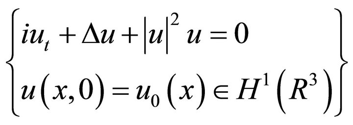
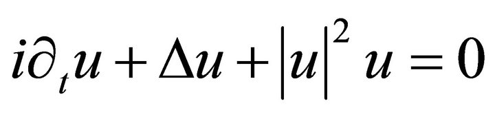
We consider the Cauchy problem for the nonlinear Schrödinger equation
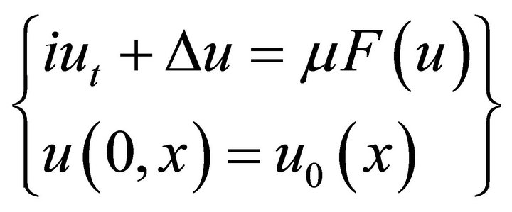 (1.1)
(1.1)
where ,
,  the solution
is a complex-valued function in 
The Equation (1.1) is called mass-critical or  critical if
 , and it is called mass-supercritical and energy-subcritical when
 .
.
The solutions to (1.1) have the invariant scaling
 (1.2)
(1.2)
Definition 1.1 (Solution) Let  such that
 . A function
  is a strong solution to (1.1)
if and only if it belongs to , and for all
  satisfies the integral equation
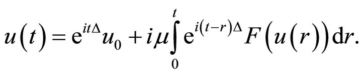 (1.3)
(1.3)
A function  is a weak solution to (1.1)
if and only if , and for all
satisfies the integral Equation (1.3).
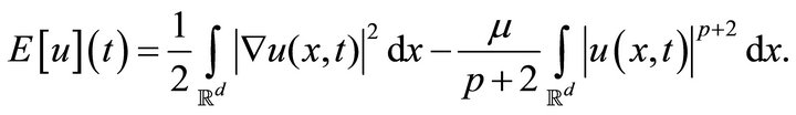
The solutions to (1.1) have the mass
where
Energy  where,
Definition 1.2 The problem (1.1) is locally wellposed in  if for any
  there exist a time
  and an open ball
  in
in  such that
 , and a subset
  of
of , such that for each
  there exists a unique solution
  to the Equation (1.3), and furthermore, the map
  is continuous from
 . If
. If ![]() can be taken arbitrarily large
can be taken arbitrarily large , the problem is globally wellposed.
Definition 1.3 A global solution  to (1.1) is scattering in
  as
as  if there exists
  such that
Similarly, we can define scattering in  for
for .
.
For more definition of critical case see [1-3].
In this paper we discuss stability theory of the mass critical, mass-supercritical and energy-subcritical of solution to the nonlinear Schrödinger equation. In section three we discuss the stability of the mass critical solutions and in section four mass-supercritical and energysub-critical solutions are discussed.
Theorem 1.1 Let  and
and . Then there exists a unique maximal-lifespan solution
 ![]()
 to (1.1) with
  and initial data
 . Moreover:
1) The interval  is an open subset of
 .
.
2) For all , we have
  so, we define
 .
.
3) If the solution ![]() does not blow up forward in time, then
does not blow up forward in time, then , and moreover
 ![]() scatters forward in time to
scatters forward in time to  for some
 . Converselyif
  then there exists a unique maximallifespan solution
 ![]() which scatters forward in time to
which scatters forward in time to .
.
4) If the solution u does not blow up backward in time, then  and moreover
 ![]() scatters backward in time to
scatters backward in time to  for some
 . Conversely, if
 then there exists a unique maximallifespan solution
 ![]() which scatters backward in time to
which scatters backward in time to .
.
5) If  where a constant
  depending only on
 ![]() then
then
 .
.
In particular, no blowup occurs and we have global existence and scattering both ways.
6) For every  and
and  there exists
  With property: if
  is a solution (not necessarily maximal-lifespan) such that
 and
and ,
,  are such that
 , then there exists a solution
 with
with  such that
and  for all
 .
.
For proof: See [4-6].
Now in the following we will discuss Standard local well-posedness theorem.
Theorem 1.2 Let ,
,  and let
 Assume that
  if
if ![]() is not an even integer. Then there exists
is not an even integer. Then there exists  such that if between
  and
and  there is a compact interval containing zero such that
 (1.4)
(1.4)
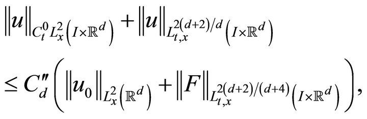
then there exists a unique solution u to (1.1) on . Furthermore, we have the bounds
 (1.5)
(1.5)
 (1.6)
(1.6)
 (1.7)
(1.7)
where  for the closure of all test functions under this norm.
2. Strichartz Estimate
In this section we discus some notation and Strichartz estimate.
2.1. Some Notation
We write  anywhere in this work whenever there exists a constant
 ![]() independent of the parameters, so that
independent of the parameters, so that . The shortcut
  denotes a finite linear gathering of terms that “look like” X, but possibly with some factors changed by their complex conjugates.
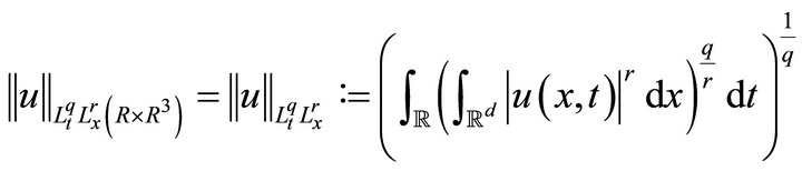
We start by the definition of space-time norms
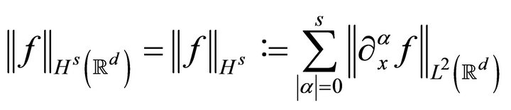
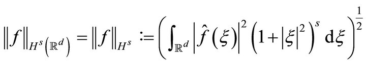
The inhomogeneous Sobolev norm  (when
(when ![]() is an integer) is defined by:
is an integer) is defined by:
When s is any real number as
The homogeneous Sobolev norm  defines as:
For any space time slab We use
  to denote the Banach space of function
  whose norm is
With the usual adjustments when  or
or  is equal to infinity. When
  we abbreviate
  as
as .
.
A Gagliardo-Nirenberg type inequality for Schrö- dinger equation the generator of the pseudo conformal transformation  plays the role of partial differentiation.
2.2. Strichartz Estimate
Definition 2.1 The exponent pair  is says the Schrödinger-admissible if
 , and
, and 
Definition 2.2 The exponent pair  is says the Schrödinger-acceptable if

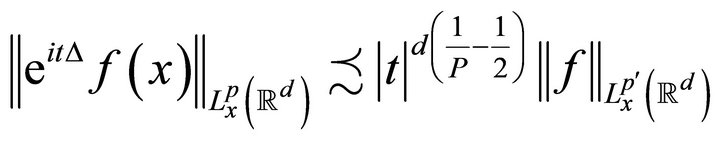
Let  be the free Schrödinger evolution. From the explicit formula
we obtain the standard dispersive inequality
 (2.1)
(2.1)
for all .
.
In particular, as the free propagator conserves the  - norm,
 (2.2)
(2.2)
For all 
If  solves the inhomogeneous Equation (1.1) for some
 and
and ![]()
in the integral.
Duhamel (1.3). Then we have
 (2.3)
(2.3)
for some constant  depending only on the dimension
![]() .
.
For some constant  depending only on
 ![]() we have the Holder inequality
we have the Holder inequality
We now return to prove Theorem 1.2.
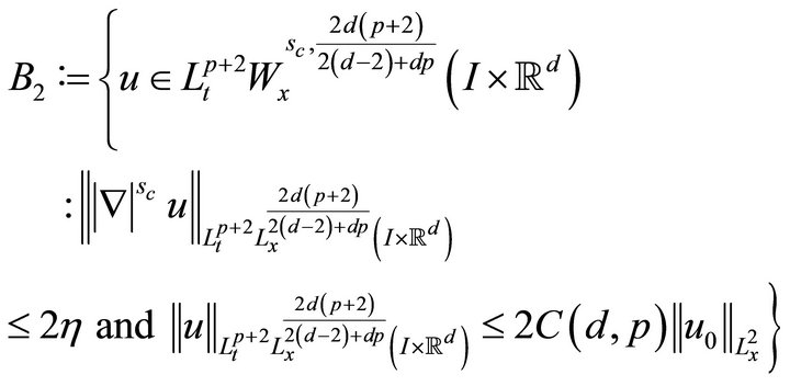
Proof Theorem 1.2 The theorem follows from a contraction mapping argument. More accurate, defined
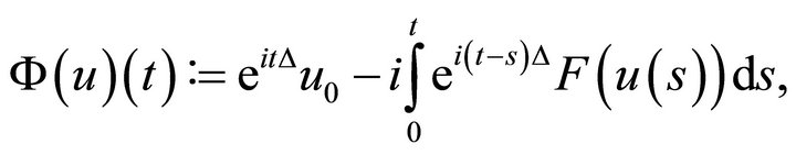
using the Strichartz estimates, we will show that the map  is a contraction on the set
  where
where

under the metric given by
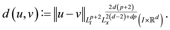
Here  denotes a constant that changes from line to line. Note that the norm appearing in the metric scales like
 . Note also that both
  and
and  are closed (and hence complete) in this metric.
Using the Strichartz inequality and Sobolev embedding, we find that for 
And similarly,
Arguing as above and invoking (1.4), we obtain
Thus, choosing  suciently small, we see that for
 , the functional
  maps the set
  back to itself. To see that
  is a contraction, we repeat the above calculations to obtain
Therefore, choosing  even smaller (if necessary), we can ensure that
  is a contraction on the set
 . By the contraction mapping theorem, it follows that
  has a fixed point in
 . Furthermore, noting that
  maps into
  (not just
 ). We now turn our attention to the uniqueness. Since uniqueness is a local property, it enough to study a neighbourhood of
  By Definition of solution (and the Strichartz inequality), any solution to (1.1) belongs to
  on some such neighbourhood. Uniqueness thus follows from uniqueness in the contraction mapping theorem.
The claims (1.6) and (1.7) follow from another application of the Strichartz inequality. □
Remark 2.1 By the Strichartz inequality, we know that
Thus, (1.4) holds with  for initial data with suciently small norm instead that, by the monotone convergence theorem, (1.4) holds provided
  is chosen suciently small. Note that by scaling, the length of the interval
  depends on the fine properties of
 , not only on its norm.
3. Stability of the Mass Critical
In this section we discuss the stability theory at mass critical case. Consider the initial-value problem (1.1)
with  .An important part of the local well-posedness theory is the study of how the strong solutions built in the past subsection depend upon the initial data. More accurate, we want to know if the small perturbation of the initial data gives small changes in solution. In general, we take care in developing a stability theory for nonlinear Schrödinger Equation (1.1). Even though stability is a local question, it plays an important role in all existing treatments of the global well-posedness problem for nonlinear Schrödinger equation at critical case, for more see [7]. It has also proved useful in the treatment of local and global questions for more exotic nonlinearities [8,9]. In this section, we will only discus the stability theory for the mass-critical NLS.
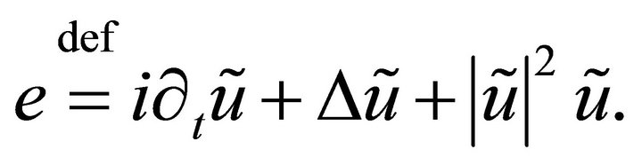
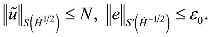
Lemma 3.1 Let  be a compact interval and let
  be an approximate solution to (1.1) meaning that
for some function![]() . Suppose that
. Suppose that
 (3.1)
(3.1)
for some positive constant . Let
. Let  and let
  be such that
 (3.2)
(3.2)
for some . Suppose also the smallness conditions
 (3.3)
(3.3)
 (3.4)
(3.4)  (3.5)
(3.5)
for some  where
where  is a small constant. Then, there exists a solution
 ![]() to (1.1) on
to (1.1) on  with initial data
  at time
  satisfying
 (3.6)
(3.6)
 (3.7)
(3.7)
 (3.8)
(3.8)
 (3.9)
(3.9)
Proof: By symmetry, we may assume . Let
. Let . Then
 ![]() satisfies the initial value problem
satisfies the initial value problem

For  we define
By (3.3),
 (3.10)
Furthermore, by Strichartz, (3.4), and (3.5), we get
 (3.11)
Combining (3.10) and (3.11), we obtain
A standard continuity argument then shows that if  is taken sufficiently small,
which implies (3.9). Using (3.9) and (3.11), we obtained (3.6). Furthermore, by Strichartz, (3.2), (3.5), and (3.9),
which establishes (3.7) for  sufficiently small.
To prove (3.8), we use Strichartz, (3.1), (3.2), (3.9), and (3.3):
Choosing  sufficiently small, this finishes the proof. □
Based on the previous result, we are now able to prove stability for the mass-critical NLS.
Theorem 3.2 Let  be a compact interval and let
  be an approximate solution to (1.1) in the sense that

for some function![]() . Assume that condition (3.1) in Lemma 3.1 holds and
. Assume that condition (3.1) in Lemma 3.1 holds and
 (3.12)
for some positive constant . Let
. Let  and let
  obey (3.2) for some
 . Furthermore, suppose the smallness conditions (3.4), (3.5) in Lemma 3.1. For some
  where
where
 is a small constant. Then, there exists a solution
 ![]() to (1.1) on
to (1.1) on  with initial data
  at time
  satisfying
 (3.13)
 (3.14)
 (3.15)
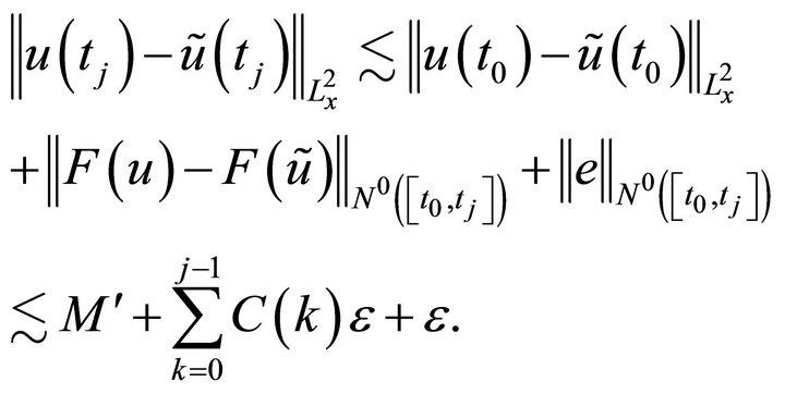
Proof: Subdivide  into
into  subintervals
  such that
where  is as in Lemma 3.1. We replaced
  by
by  as the mass of the difference
  might grow slightly in time. By choosing
  sufficiently small depending on
  and
and , we can apply Lemma 3.1 to obtain for each
  and all
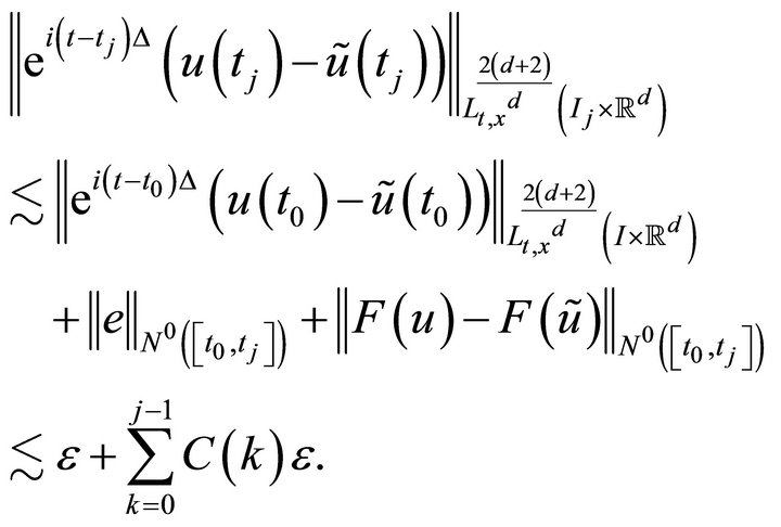
Provided, we can prove that their counterparts of (3.2) and (3.4) hold with replace ![]() by
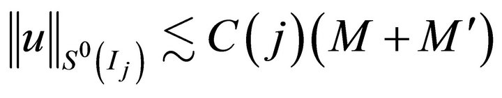
by![]() . To verify this, we use an inductive argument. By Strichartz, (3.2), (3.5), and the inductive hypothesis,
. To verify this, we use an inductive argument. By Strichartz, (3.2), (3.5), and the inductive hypothesis,
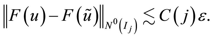
Similarly, by Strichartz, (3.4), (3.4), and the inductive hypothesis,
Choosing  sufficiently small depending on
  and
and , we can ensure that hypotheses of Lemma 3.1 continue to hold as j varies. □
Lemma 3.3 (Stability) Fix ![]() and
and![]() . For every
. For every  and
and  there exists
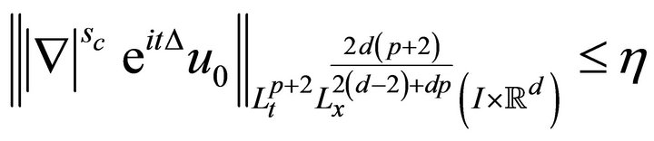
  with the property: if
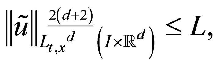
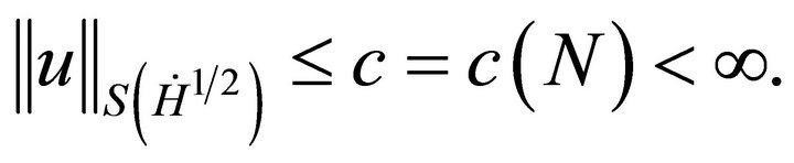
  is such that
  and that
 ![]() approximately solves (1.1) in the sense that
approximately solves (1.1) in the sense that
 . (3.16)
And ,
,  are such that
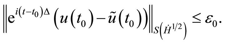
Then there exists a solution  to (1.1) with
  such that
 .
.
Note that, the masses of ![]() and
and  do not appear immediately in this lemma, although it is necessary that these masses are finite. Similar stability results for the energy-critical NLS (in
 ) instead of
 , of course) have appeared in [10-14]. The mass-critical case it is actually slightly simpler as one does not need to deal with the existence of a derivative in the regularity class. For more see [15].
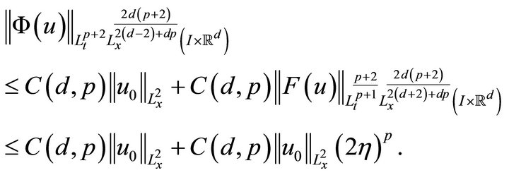
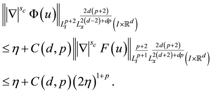
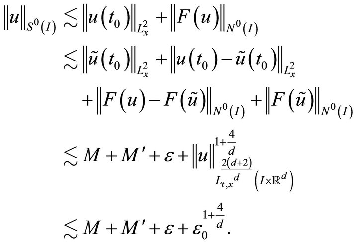
Proof: (Sketch) First let prove the claim when  is suciently small depending on
![]() . Let
. Let  be the maximal-lifespan solution with initial data
 . Writing
  on the interval
 , we see that

and
 .
.
Thus, if we set
by the triangle inequality, (2.3), and (3.16), we have
hence, by (2.4) and the hypothesis ,
,
where  depends only on
![]() . If
. If  is suciently small depending on
![]() , and
, and ![]() is suciently small depending on
is suciently small depending on ![]() and
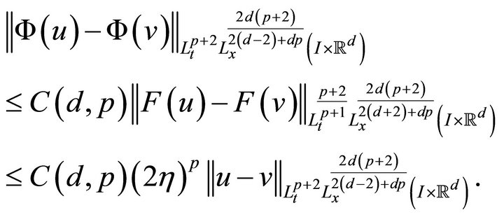
and![]() , then standard continuity arguments give
, then standard continuity arguments give  as desired. To deal with the case when
  is large, simply iterate the case when
  is small (shrinking
![]() ,
, ![]() repeatedly) after a subdivision of the time interval
repeatedly) after a subdivision of the time interval .
.
4. Stability of the Mass-Supercritical and Energy-Subcritical
In this section we discuss the Stability theory of the mass-supercritical and energy-subcritical to the nonlinear Schrödinger equation. Consider the initial-value problem (1.1) with  and
and  we chose
 .
.
In this case the initial-value problem  is locally well-posed in
 . Now we rewrite (1.1) as
 (1.1)*
We discuss the stability by the following proposition. Before beginning we need define the Kato inhomogeneous Strichartz estimate. See [16]
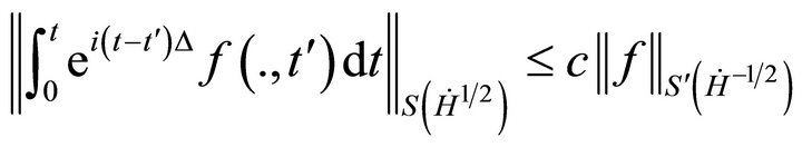 (4.1)
(4.1)
Proposition 4.1 For each  there exists
  and
and  such that the following holds.
Let  and solve
 .
.
Let  for all
  and define
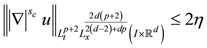
If
And
 (4.2)
(4.2)
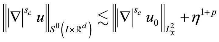
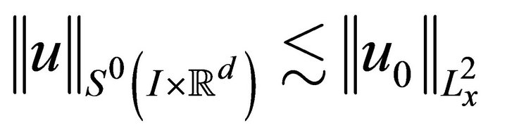
Then
Proof: Let w be defined by 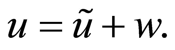 then
then ![]() solves the equation
solves the equation
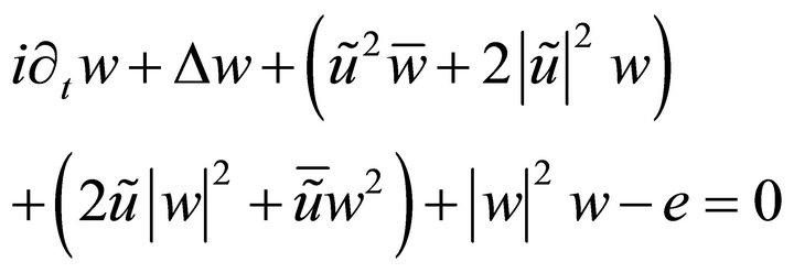 (4.3)
(4.3)
since .Can be divided
  into
into
 in intervals
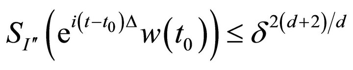
  Such that for all
 , the quantity
 , is Appropriate small
(δ to be selected below).
Integration (4.3) with initial time ![]() is
is
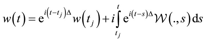 (4.4)
(4.4)
where
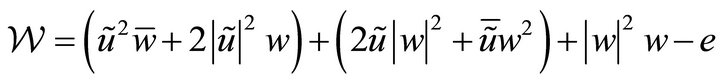 .
.
Applying the Kato Strichartz estimate (4.1) on , to obtain
 . (4.5)
Note that
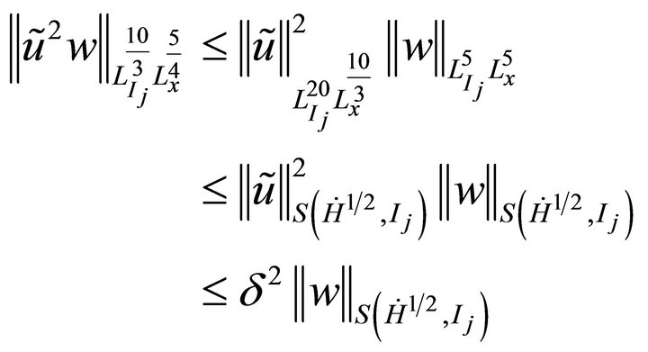 .
.
Similarly,
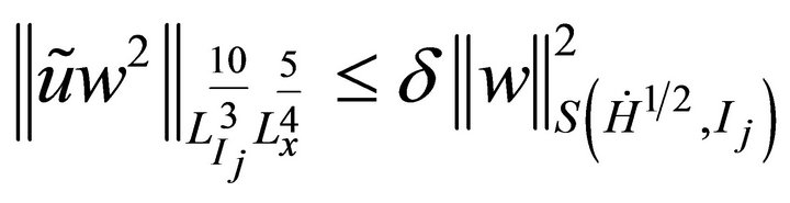
and
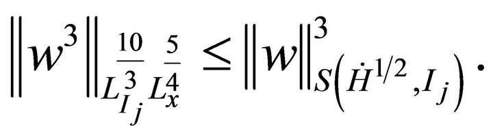
Substituting the above estimates in (4.5), to get,
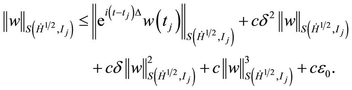 (4.6)
(4.6)
As long as
and
 (4.7)
(4.7)
We obtain
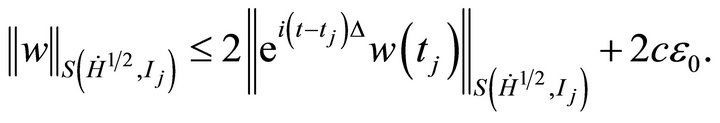 (4.8)
(4.8)
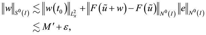
Taken now  in (4.4) and apply
  to both sides to obtain
 (4.9)
(4.9)
Since the Duhamel integral is restricted to by again applying the Kato estimate, similarly to (4.6) we obtain,
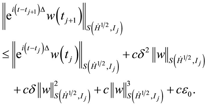
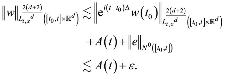
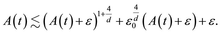
By (4.8) and (4.9), we bound the Former of expression to obtain

Start iterates with , we obtain
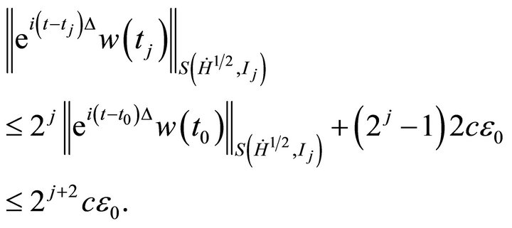
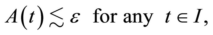
To absorb the second part of (4.7) for all intervals 
 we require
 (4.10)
We review that the dependence of parameters δ is an absolute constant chosen to meet the first part of (4.7). The inequality (4.10) determines how the small  needs to be taken in terms of
  (and thus, in terms of
 ). We were given
  which then determined
  □
□
REFERENCES
- S. Keraani, “On the Blow-Up Phenomenon of the Critical Nonlinear Schrödinger Equation,” Journal of Functional Analysis, Vol. 235, No. 1, 2006, pp. 171-192. doi:10.1016/j.jfa.2005.10.005
- R. Killip, M. Visan and X. Zhang, “Energy-Critical NLS with Quadratic Potentials,” Communications in Partial Differential Equations, Vol. 34, No. 12, 2009, pp. 1531- 1565.
- T. Tao, M. Visan and X. Zhang, “Global Well-Posedness and Scattering for the Mass-Critical Nonlinear Schrö- dinger Equation for Radial Data in High Dimensions,” Duke Mathematical Journal, Vol. 140, No. 1, 2007, pp. 165-202.
- T. Cazenave, “Semilinear Schrödinger Equations,” Courant Lecture Notes in Mathematics, New York University, 2003.
- T. Cazenave and F. B. Weissler, “Critical Nonlinear Schrödinger Equation,” Nonlinear Analysis: Theory, Methods & Applications, Vol. 14, No. 10, 1990, pp. 807-836. doi:10.1016/0362-546X(90)90023-A
- Y. Tsutsumi, “L2-Solutions for Nonlinear Schrödinger Equations and Nonlinear Groups,” Funkcial Ekvac, Vol. 30, No. 1, 1987, pp. 115-125.
- R. Killip and M. Visan, “Nonlinear Schrödinger Equations at Critical Regularity,” Clay Mathematics Proceedings, Vol. 10, 2009.
- T. Tao, M. Visan and X. Zhang, “The Nonlinear Schrö- dinger Equation with Combined Power-Type Nonlinearities,” Communications in Partial Differential Equations, Vol. 32, No. 7-9, 2007, pp. 1281-1343.
- X. Zhang, “On the Cauchy Problem of 3-D EnergyCritical Schrödinger Equations with Sub-Critical Perturbations,” Journal of Differential Equations, Vol. 230, No. 2, 2006, pp. 422-445.
- J. Colliander, M. Keel, G. Stafflani, H. Takaoka and T. Tao, “Global Well-Posedness and Scattering in the Energy Space for the Critical Nonlinear Schrödinger Equation in R3,” Analysis of PDEs.
- C. Kenig and F. Merle, “Global Well-Posedness, Scattering, and Blowup for the Energy-Critical, Focusing, Non-Linear Schrödinger Equation in the Radial Case,” preprint.
- E. Ryckman and M. Visan, “Global Well-Posedness and Scattering for the Defocusing Energy-Critical Nonlinear Schrödinger Equation in R1 + 4,” American Journal of Mathematics.
- T. Tao and M. Visan, “Stability of Energy-Critical Nonlinear Schrödinger Equations in High Dimensions,” Electronic Journal of Differential Equations, Vol. 2005, No. 118, 2005, pp. 1-28.
- M. Visan, “The Defocusing Energy-Critical Nonlinear Schrödinger Equation in Higher Dimensions,” Duke Mathematical Journal.
- T. Tao, M. Visan and X. Zhang, “Minimal-Mass Blowup Solutions of the Mass-Critical NLS,” Forum Mathematicum, Vol. 20, No. 5, 2008, pp. 881-919. doi:10.1515/FORUM.2008.042
- D. Foschi, “Inhomogeneous Strichartz Estimates,” Advances in Difference Equations, Vol. 2, No. 1, 2005, pp. 1- 24.