Open Journal of Biophysics
Vol.2 No.3(2012), Article ID:21417,8 pages DOI:10.4236/ojbiphy.2012.23009
On the Dynamic Equilibrium in Homeostasis
1Department of Complementary Medicine, University of Pécs, Pécs, Hungary
2Department of Biotechnics, St. Istvan University, Godollo, Hungary
Email: Szasz.Andras@gek.szie.hu
Received February 19, 2012; revised March 21, 2012; accepted April 9, 2012
Keywords: Homeostasis; Entropy; Bioscaling; Aging; Competing Feedback-Signals; Multiscaling Entropy; MSE
ABSTRACT
We studied the homeostatic equilibrium of the healthy organism. The homeostasis is controlled by oppositely effective physiologic feedback signal-pairs in various time-scales. We show the entropy of every signal in this state is identical and constant: SE = 1.8. The controlling physiological signals fluctuate around their average values. The fluctuation is time-fractal, (pink-noise), which characterizes the homeostasis. The aging is the degradation of the competing pairs of signals, decreasing the complexity of the organism. This way, the color of the noise gradually changes to brown. A special scaling process occurs during the aging: the exponent of the frequency dependence of the power density function grows in this process from 1 to 2, but the homeostasis of the system is unchanged.
1. Introduction
Life is based on energetically open systems, where the environmental conditions determine it as equilibrium. The living equilibrium is the homeostasis. The actual homeostatic state is definitely “constant” despite its energetically open status. The normal healthy state of any living system is in homeostasis, which is not static, but dynamically change in time, forming a relatively stable state. This relative stability makes it possible to recognize the various individuals despite the fact that millions of their cells actually vanish and millions of those are reborn. The homeostasis is controlled by numerous negative feedback loops [1,2], creating both the microand macro-structures in equilibrium.
The disease breaks the relative equilibrium, risks the relative stability of the system. The system tries to reestablish the homeostasis by enhancing the negative feedback control. The physiology tries to compensate and correct the damage.
The natural therapy must help the body’s internal corrective actions to reestablish the healthy state. Recognizing the disease, most of the medical approaches act with changes of the conditions (diets, medicaments, other supplies) trying to constrain the body back to the previously working equilibrium. However, in many cases, it works against the natural homeostasis, the constrained action induces new homeostatic negative feedbacks from the living object. The living organism starts to fight against our constraints together with the fight against the disease [3]. This is the problem of the classical hyperthermia, which introduces a new constrained effect, the heating out from the natural homeostasis. This constraint induces physiological feedback, forcing the body to fight on “double front”: against the disease and against the action of the heat.
This controversial situation happens for example in case of the classical hyperthermia in oncology, when the constrained massive temperature change is physiologically down-regulated (or at least the physiology works against it by the systemic [like blood-flow] and local [like heat-shock] [protein (HSP)] reactions) [4]. Oncothermia disclaims the old approach, introducing a new paradigm: with the application of micro-heating it induces considerably less physiological feedback to work against the action, and with the application of the electric field it uses such an effect, for which the body has no physiological answer. With this new paradigm, oncothermia helps the natural feedback mechanisms to reestablish the healthy state [4]. This simple example shows the crucial role of the homeostasis in the curative processes.
2. Homeostasis and Entropy
To characterize the homeostatic equilibrium we may introduce a special entropy-definition.
There are various proposals to calculate the entropy of finite data-series, which are coherent with the Shannontype entropy [5]. Measuring complexity of time-series was introduced the Richman-Moorman-entropy [6].
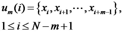
Define a time-series of N-sampling with  . Choose m-length vectors from this:
 (1)
(1)
and use the maxima of the absolute deviation of the components for characterizing the distances between the vectors:
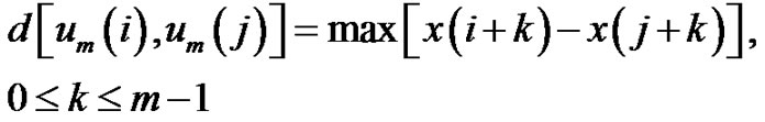 (2)
(2)
The  and
and  vectors are r-neighbors when their distance is less than r.
The Richman-Moorman-entropy is the negative logarithm of that conditional probability that the vectors remain r-neighbors when we add a new sample-point to the time-series so the length of the vectors are elongated to . Consequently:
 (3)
(3)
Denote the number of 
 vectors which have closer distance than r from
  by
by . Define the probability that the
  vector is in the neighborhood of
  at r-radius:
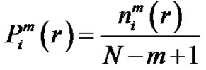 (4)
(4)
While the probability that the  vector is in the r-radii neighborhood of
 :
:
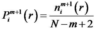 (5)
(5)
From these, the conditional probability is:
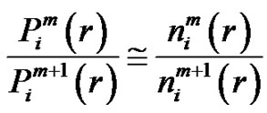 (6)
(6)
and hence the Richman-Moorman-entropy:
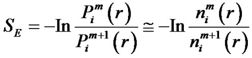 (7)
(7)
The  and
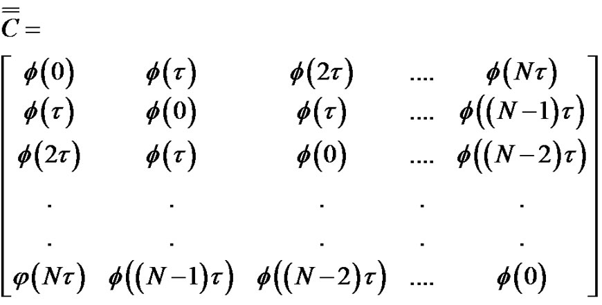
and  quantities in Equation (7) could be determined from the probability distribution function of the vectors. Analyzing the multiple-scale entropy of physiological signals the Richman-Moormanentropy was applied [7]. Supposing that the Gauss-type pink-noise at physiologic signals is a good approximation due to the central limit theorem [8]. The covariance matrix is necessary for characterizing the multidimensional Gauss-distribution. In case of the Gauss-pink-noise, the covariance matrix could be determined from the power spectrum, and on this basis the entropy as well.
The definition of the covariance matrix of random N-variables is:
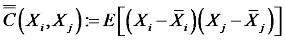 (8)
(8)
The diagonal of the covariance matrix contains the deviations of the random variables. The covariance matrix is hermitic, symmetric with real values, consequently it could be diagonal-transformed, and its characteristic equation with λi eigenvalues:
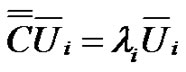 (9)
(9)
Hence:
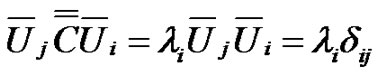 (10)
(10)
Consequently, forming a  matrix from the eigenvectors as columns will be diagonal:
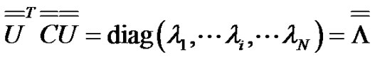 (11)
(11)
Due to the transformation:
 (12)
(12)
the transformed random variables:
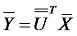 (13)
(13)
have the same covariance matrix. Consequently, the deviation of  transformed random variables are:
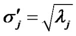 (14)
(14)
On the other hand, the probability density function of the N-dimensional noise with Gauss-distribution is:
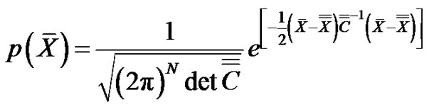 (15)
(15)
from where the distribution function of the transformed random variable is:
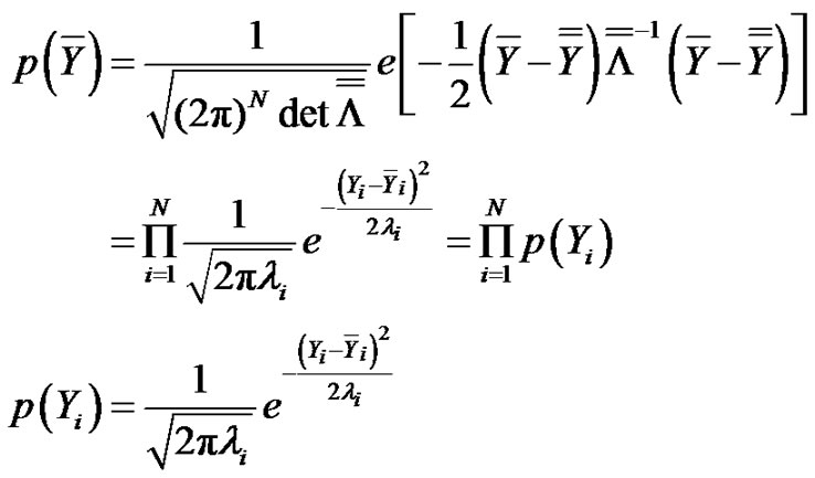 (16)
(16)
Calculating the covariance matrix, the power density of pink-noise:
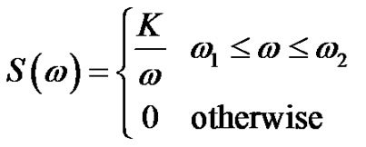 (17)
(17)
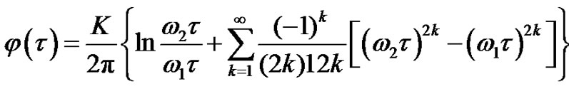
From Equation (17) the autocorrelation function could be determined by the Wiener-Khinshin-theorem [9]:
 (18)
(18)
where isthe integral-cosine function and
  is the Euler constant. Hence:
 (19)
(19)
The connection of the covariance matrix and the autocorrelation function for the ergodic processes (like the pink noise) is Equation [7]:
 (20)
(20)
From these the entropy of pink nose was obtained [7]:
 (21)
(21)
So, this analysis proved the scale-independency of pinknoise in a definite interval of the signals. The multiscale entropy analysis (MSE, [7]) is applied to analyze various physiological signals [10]. Its application made on a discrete one-dimensional time-series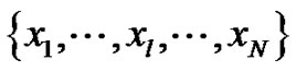 .
.
From this a consecutive coarse-grained  timeseries is constructed with
  scale-factor. With averaging or smoothing (filtering) another time series can be presented. Noises with different
  scales could be constructed this way:
 (22)
(22)
and we determine the entropy of all the coarse-grained time-series. This is the Multiscale Entropy analysis (MSE) [7] method. Applying the above process for pinkand white-noises, and the entropy vs the applied scale factors (number of the members of the actual averaging) had different functions. The smoothing (filtering, cutting the high-frequencies) is irrelevant in case of the pinknoise. When the original was pink, the entropy remains constant on all scales in a very wide range of limits. The entropy of the white-noise is decreased by the growing scale-factors, in consequence of the very short correlation; but its entropy is high at the scales, less than 4, due to the short range correlations. The short correlation is weak, but the long is strong for the pink-noise.
3. Physical Consequences of MSE Results
From physical point of view, the scaling of a discrete time series is a filtering process, which rejects some high-frequency components of the noise. The largest band-width of the noise is at scale 1. Gradually jumping onto a higher scaling, the average of the high-frequency components is more and the bandwidth decreases. The highest frequency in the signal could be estimated by the Shannon’s sampling-theorem: the largest frequency appearing in the noise is the half of the sampling frequency. In consequence: in case of scale factor 2 the half, in case of scale factor n the n-th part of the highest frequency determines the bandwidth. The same is valid in the lowest frequency-limit of the bandwidth.
The length of the data-series is the function of the registration time. When  is the sampling time and N is the size of the data-series, the time of registering is
 . The reciprocal value of this time is the smallest frequency in the signal, so it is the lower boundary of the bandwidth. Due to the decreasing length of the data-series by scaling, the lower frequency-limit of the bandwidth is growing (see Figure 1).
The Richman-Moorman-entropy of the time-series shows a “holographic-like” structure of the pink noise: the truncation of the noise does not change its entropy.
The Richman-Moorman-entropy of course has physical meaning in the same way as in the Shannon-entropy (they are coherent). Multiplying the Richman-Moorman-

Figure 1. Narrowing the bandwidth by scaling.
entropy by the Boltzmann constant, the physical entropy of the registered signal is constructed. The entropy of a system is the function of state; so it is a function of the state-variables, among which the energy is one of the most important variables. In our present case the energy of the system is the sum of the energy-values of the Fourier components of the registered noise. In consequence, the entropy of the signals formed from pink noise does not change by its decreasing energy. This case is seen in the thermodynamics: the entropy of the system in the equilibrium thermodynamics has extremum in function of energy, which means that the subsystems having thermodynamic equilibrium could exchange energies by fluctuations without changing the entropy of the system. It seems that a similar situation exists in case of such stochastic systems, which emits pink noise. If this analogy is valid, the subsystems can exchange considerable energy without changing the entropy of the system. Introducing a type of function like the temperature is impossible, because the entropy here isn’t additive, as the entropies of all the pink-noise systems are equal. Here the entropy is more intensive than extensive parameter in the description of the system.
4. Network Control of the Homeostasis
The mesenchyme, which is 25% of the human body, has an important role of forming homeostasis in the organism [11]. It is a loose connective tissue with an undifferentiated type [12]. The pink-noise with entropy SE = 1.8 characterizes the homeostasis like an intensive parameter. This intensivity is valid for every physiologic signal and for all the organs, the SE = 1.8 is a universal constant for the living body.
The cellular functions like supplies and filtering are mediated by the mesenchyme, which represents a transmitter between the blood-capillaries and the cells. The mesenchyme is a ground substance matrix for the cells, it is an ordered set of meshwork of connective species like highly polymerized hydro-carbonates, gucosaminoglycans, ologasacharid-chans connected to proteins, proteoglycans, and structure-glycoproteins, meshed by the dendrites of cellular glycocalix and by the extracellular matrix.
Mesenchyme has a trimodal function: cellular, humoral and neural. The cellular function brings the chemical equilibrium of connective tissue together with reticuloendothel cells. The humoral function controls the transport processes through the capillaries and lymphnetwork. This transport mechanism ensures the communication with far away systems. The neural function is responsible for the functional connection with all other parts of the organism. The three levels are different in their ranges: the cellular is local, the humoral is mesoscopic and the neural is global (systemic) interaction in the body. Due to the slow transport processes, the humoral effects are slow, while the neural is speedy.
The information control is effective by assistance of the neural system, of the cellular transport (hormones, enzymes, apoptosis, “social” signals) and of the humoral by blood and lymph transports too. The cell is the quickest to react. All the controlling mechanisms are operated by a pair of opposite signals: upand down-regulation of the actual process. This is valid in all the time-scales having numerous pairs to form the physiological signals. The three levels are connected to each other by the mesenchyme.
The homeostasis is determined by the equilibrium of the large number of opposite pairs. As an example, we describe the proliferation homeostasis. There is a mechanism, which replaces the aged, harmed or too stressful cells. This process, which again the equilibrium of the opposite driving forces, stabilizes the final size of the organs. The opposite processes are the annihilation (apoptosis driven by the programmed cell death) and creation (cell division driven by growth factors). The two sides are in equilibrium in healthy state. When this equilibrium vanishes, the system cannot work well, that is the illness. When the apoptosis starts to dominate that could be an autoimmune disease, when the creation determines the process, the tumor is the result. The complexity of the system (which is characterized by the number of the opposing pairs) is the basic of the proper work, allows the system to accommodate properly to the environmental challenges. The acting signal-pairs are connected and coupled to each other, forming a unified complex system.
The above shown proliferation homeostasis works on the renewing of the cellular system, but one cell has to be annihilated giving place for the new-born one keeping the complete function in equilibrium (homeostasis). The equilibrium of this complex system could be described by fractal physiology [13-16] and bio-scaling [17-19]. This complexity is mirrored in the four dimensional description of the living state [20], which is valid in all scales of the life [21].
The complex network of the regulating pairs with opposite actions is the basis of the Traditional Chinese Medicine (TCM) and philosophy too (Yin-Yang pairs). The complexity means that the system cannot be simple additionally composed from their parts, the parts alone do not carry the function, which they have in the complete complex system. The couplings and interactions between the controlling pairs could explain the multifunctional behavior of tuning a single controlling pair, so the consequences of one external retuning of the balance could lead to various results.
We present this interaction of the sample of the proliferation homeostasis again. One of the functions of the mesenchyme is humoral by the transport of nutrients. When the oxygen supply is insufficient in an organ (hypoxia for example by the extreme utilization of a group of muscles), the conditions of the cells become hypoxic. The cells destroyed by the hypoxia release such chemicals into the extracellular electrolyte, which dissolve the endothelial cellular connections in the capillaries, breaking their adherent (cytoskeleton) connections. This ignites the first step of the angiogenesis, when the structure of the endothelial cells in the vessel-wall changes, the vascular tone reduces and the permeability of the vessel-wall increases. The increased permeability provides better oxygen and nutrient supply to the tissue. In the second stage of the angiogenesis protecolis-enzymes evolve, making the extracellular electrolyte less viscose, giving possibility for the cells to have higher motility. The effect of the Vascular Endothelial Growth Factor (VEGF) is inducing cellular division and helping the chemotactically driven migration by the gradients of the growth factors. It starts building up a primitive network of vessels.
The fourth step of angiogenesis is the maturation, when the extracellular matrix is reconstructed, the cellular connections reestablished, and the vessel-wall builds its stable final form. In this step the angiopoietin molecules have the duty to connect the primitive just-born capillarity vessels into the existing network. The proper physiological function (transport) of the new vessel is not enough to finish the job, transport must be given where the nutrient + oxygen supply is requested.
The vessels are built up by a morphogenetic network, constructed by the gradients of the growth factors and by the electric potential gradients, which occur in the more negative daughter-cells than their matured counterpart (see Figure 2).
The potential gradient determines the direction of growth and the equilibrium is constructed by the dynamic control of the network of opposing pairs of actions, which is built up by the well determined scaling [22], ensure the proper equilibrium energy supply of the newly reborn complex system.
The deterministic way of the control cannot be accu-
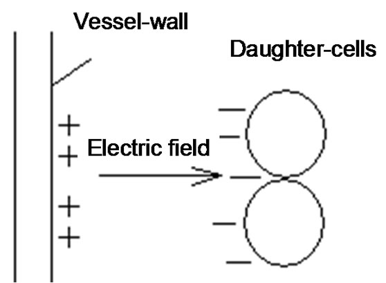
Figure 2. Construction of electric potential gradient by angiogenesis.
rate and stable enough, with appropriate processing velocity, so the process is not deterministic. There is a crucial role of the random processes also to make the control optimal, not to use unnecessary accuracy and waste energy to control the system. The aims of the homeostasis are to safeguard the cellular functions and to assure the constant life-conditions for these smallest units. The environmental parameters must be kept in a tolerable band, the fluctuations of the actual values must not go over a definite limit for a longer time. These thresholds keep the average of the parameters constant in time, but due to the given band-width the deviation must also be fixed (see Figure 3).
The structure of fluctuations is essential in this stochastic process. We show in the next the time-fractal fluctuations satisfy the above request of the homeostasis. Time-fractal is the signal of stochastic control of homeostasis.
Consider the environmental signal, (see Figure 4), which is controlled by a homeostatic process is an average of various components:
 (23)
(23)
The average is the basic signal and the deviation form is the controlling error. Due to the random processes, the controlling error is a noise in the homeostasis.

Figure 3. The fluctuations must be in the definite range properly keeping the control. Consequently, the average always has to be fixed in time, and the random fluctuations remain in the band for a long-range of the time.
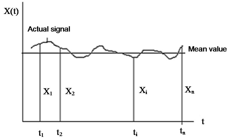
Figure 4. Homeostasis controlled parameter of the environmental signal.
Consequently the noise: (24)
(24)
where  denotes the averaging by time. The variance of the noise
 , is also time-dependent:
 (25)
(25)
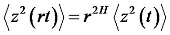
Due to the living structure, the noise has to be selfsimilar [23]. This means that the variance of the noise has a time-dependent power-function [24]:
 (26)
(26)
where the similarity exponent is always positive: . Consider the following example as
 , then the control-error variance is the linear function of the time:
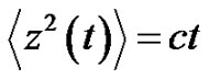 (27)
(27)
where c is constant. In this case, the error-signal is a Brownian-motion. The scaling law is in consequence of Equation (26):
 (28)
(28)
The error signal can be characterized by the spectral power density function:
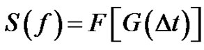 (29)
(29)
where  is the autocorrelation function of the error signal:
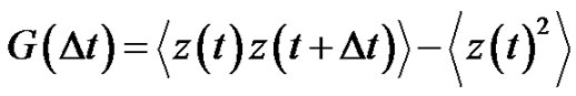 (30)
(30)
The spectral power density function for the above introduces self-similar noises:
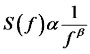 (31)
(31)
The power  is the “color” of the error signal and depends on H [25]:
 (32)
(32)
Consequently:
 (33)
(33)
Hence if the error-signal is pink noise (
 — noise), than
 (34)
(34)
Therefore, due to Equation (26), when the noise is , then its deviation is constant in time in the well chosen interval. Indeed, the probability of the error signal exists in the interval
  (where σ is the standard deviation) on the basis of the Chebishev inequality [26] is:
 (35)
(35)
Consequently, when the k is large enough, (large enough time is chosen for averaging) the probability is practically one, so the signal does not leave the chosen band. This means the system is well controlled in all times, the homeostasis is fixed, the system is regulated. The entropy of the system in this case is constant on all the scales (SE = 1.8), the signals are controlled (they are kept in a definite interval) on all scales.
When the power-spectrum of the error signal deviates from the pink-noise, has another color (for example β > 1), then its self-similar exponent will be positive, so according to Equation (26) the deviation of the error-signal will grow in time, the homeostasis of the system will be broken. In these cases extra regulation (internal or external signals) (e.g. immune reactions, transport-rearrangements, etc. or constrain treatments, therapies, etc.) is necessary to stabilize the system.
5. Aging and Scaling
Aging decreases the complexity of the system [27]. This loss means the degradation of the number of the opposite controlling pairs making the dialectic determinations. These changes could deviate the action time, the pairs act on different time-scales. Also we may assume that the quick action pairs are degraded first. All of these mean the aging is an MSE scaling, but the fluctuations of high frequency gradually disappear, the scaling possibility of the noise signal remains characteristic in normal aging cases, but shifts toward the Brownian noise (1/f2). This corresponds to the H = 1/2 in Equation (26), so the variance becomes linearly growing by time, according to Equation (27), the error-signal is a Brownian-motion, the aging suppresses the complexity [23], and the autocorrelation gradually decreases by time according to Equation (30). The scaling is a good simulation of aging, the system gradually occupies larger scale-factors. Studying the color of the noise of physiological signals to check the healthy state. We can distinguish the disease (the signal-noise is gradually shifted to white one, the correlation length decreases). On this way the loss of complexity by natural aging shifts the noise towards Brownian, opposite to the disease.
The mesenchyme is the coupling media of the action networks constructing the homeostasis. The mesenchyme is a crossing field of the homeostatic actions working like hubs for various and numerous actions. Modifying the hubs, the homeostatic control could be changed. Three main effects could act:
1) The mesenchyme over-controls. In this case the signal has to be down-regulated, purging is active [28].
2) When the signal is too low, it must be up-regulated, which is the tonization [28].
3) The signal is correct, but its deviation is too large, then a homeostatic entropy has to be produced at the hubs [28].
The outer connection points for this control are the probable acupunctural points. The living systems are energetically open, their active connections to their environment is mandatory. The special material exchange in the acupuncture points (CO2 development [29], temperature differences [30], potential differences [31]), as well as the change of the size [32] of the acupuncture point support the assumption that these connections control the hubs in the complex system.
The stimuli of the acupuncture points (controlling the active fluctuations in the homeostatic band) could be achieved by various methods, like invasive needles, like electric or laser stimuli or mechanical pressure, permanent embedding methods of acupuncture. We do not know yet the actual local processes induced by the stimuli, but probably the mechanical and electric factors make the disturbance which promotes the natural correction system to reestablish the homeostatic equilibrium. There might not be any single effect that can be blamed for the action, but various local disorders are complexly interacting, like micro-wounds making injury current, like micro-bleeding inducing Platelet-Derived GrowthFactors (PDGF), like forced cellular apoptosis and replacing division, etc. Irrespective of the realized ways of the action, the acupuncture the acupuncture could give enough disturbance to rearrange the structure of the local hub to find the homeostatic equilibrium again by selforganizing way. This is much similar to the process, when we give mechanical vibration for a bowl of cherries to arrange itself to a lower energy status with self-organization. The stimuli are active till the micro-disturbance exists [28,33]. There are examples for the stochastic disturbance inducing self-organized processes in the bioprocesses.
Forming the secondary, ternary and fourth structures of proteins operated by self-organizing way [34], and one of the functions of stress-induced proteins (Heat-Shock Proteins, HSP) is providing such disturbances for the stress-unfolded portents, where the molecules could find the lower energy state forming their normal structure again [35].
6. Conclusion
The homeostasis is the equilibrium of the living complexity. There is an entropy-definition which could characterize the system in this state. The dynamical fluctuations have pink-noise distribution, which ensures the equal deviation all over the system. The noise changes its character by disease or aging. The disease is the partial loss of the collectivity (the fluctuations are shifted towards the white noise, disordered), while the aging shifts the noise oppositely to the brown-direction (fixed routes, less adaptability, loss of complex adaptation facilities). Acupuncture probably makes changes to reestablish the pink-noise fluctuation when it is lost to white noise direction (disordered complexity), introducing disturbances in the hubs of the complex network system, making the natural rescaling of the interactions possible.
REFERENCES
- K. Sneppen, S. Krisna and S. Semsey, “Simplified Models of Biological Networks,” Annual Reviews of Biological Networks, Vol. 39, 2010, pp. 43-59. doi:10.1146/annurev.biophys.093008.131241
- G. Turrigiano, “Homeostatic Signaling: The Positive Side of Negative Feedback,” Current Opinion in Neurobiology, Vol. 17, No. 3, 2007, pp. 318-324. doi:10.1016/j.conb.2007.04.004
- A. Szasz and O. Szasz, “Oncothermia: Selective DeepHeating Far from Equilibrium, Hyperthermia: Recognition, Prevention and Treatment,” Nova Science Publishers, Hauppauge, 2011.
- A. Szasz, N. Szasz and O. Szasz, “Oncothermia—Principles and Practices,” Springer, Heidelberg, 2011.
- C. E. Shannon, “A Mathematical Theory of Communication,” Bell System Technical Journal, Vol. 27, 1948, pp. 379-423, 623-656.
- J. S. Richman and J. R. Moorman, “Physiological Time- Series Analysis Using Approximate Entropy and Sample Entropy,” American Journal of Physiology, Vol. 278, No. 6, 2000, pp. H2039-H2049.
- M. Costa, A. L. Goldberger and C. K. Peng, “Multiscale Entropy Analysis of Biological Signals,” Physical Review E, Vol. 71, No. 2, 2005, Article ID: 021906. doi:10.1103/PhysRevE.71.021906
- I. Barany and V. Van, “Central Limit Theorems for Gaussian Polytopes,” The Annals of Probability, Vol. 35, No. 4, 2007, pp. 1593-1621. doi:10.1214/009117906000000791
- http://mathworld.wolfram.com/Wiener-KhinchinTheorem.html
- R. A. Thuraisingham and G. A. Gottwald, “On Multiscale Entropy Analysis for Physiological Data,” Physica A: Statistical Mechanics and Its Applications, Vol. 366, 2006, pp. 323-332. doi:10.1016/j.physa.2005.10.008
- W. J. Rea and K. Patel, “The Physiologic Basis of Homeostasis,” In: W. J. Rea and K. Patel, Eds., Reversibility of Chronic Degenerative Disease and Hypersensitivity, CRC Press, Taylor and Francis Group, LLC, Boca Raton, 2010.
- J. M. Strum, L. P. Gartner and J. L. Hiatt, “Cell Biology and Histology,” Lippincott Williams & Wilkins, Hagerstwon, 2007.
- W. Deering and B. J. West, “Fractal Physiology,” IEEE Engineering in Medicine and Biology, Vol. 11, No. 2, 1992, pp. 40-46. doi:10.1109/51.139035
- B. J. West, “Fractal Physiology and Chaos in Medicine,” World Scientific, Singapore City, 1990.
- J. B. Bassingthwaighte, L. S. Leibovitch and B. J. West, “Fractal Physiology,” Oxford University Press, Oxford, 1994.
- T. Musha and Y. Sawada, “Physics of the Living State,” IOS Press, Amsterdam, 1994.
- J. H. Brown and G. B. West, “Scaling in Biology,” Oxford University Press, Oxford, 2000.
- J. H. Brown, G. B. West and B. J. Enquis, “Yes, West, Brown and Enquist’s Model of Allometric Scaling Is Both Mathematically Correct and Biologically Relevant,” Functional Ecology, Vol. 19, No. 4, 2005, pp. 735-738. doi:10.1111/j.1365-2435.2005.01022.x
- G. B. West and J. H. Brown, “The Origin of Allometric Scaling Laws in Biology from Genomes to Ecosystems: Towards a Quantitative Unifying Theory of Biological Structure and Organization,” Journal of Experimental Biology, Vol. 208, 2005, pp. 1575-1592. doi:10.1242/jeb.01589
- G. B. West, J. H. Brown and B. J. Enquist, “The Four Dimension of Life: Fractal Geometry and Allometric Scaling of Organisms,” Science, Vol. 284, No. 5420, 1999, pp. 1677-1679. doi:10.1126/science.284.5420.1677
- G. B. West, W. H. Woodruf and J. H. Born, “Allometric Scaling of Metabolic Rate from Molecules and Mitochondria to Cells and Mammals,” Proceedings of the National Academy of Sciences of the USA, Vol. 99, Suppl. 1, 2002, pp. 2473-2478. doi:10.1073/pnas.012579799
- G. B. West, J. H. Brown and B. J. Enquist, “Life’s Universal Scaling Law,” Physics Today, Vol. 57, No. 9, 2004, pp. 36-42. doi:10.1063/1.1809090
- A. L. Goldberger, L. A. N. Amaral, J. M. Hausdorff, P. C. Ivanov, C.-K. Peng and H. E. Stanley, “Fractal Dynamics in Physiology: Alterations with Disease and Aging,” Proceedings of the National Academy of Sciences of the USA, Vol. 99, Suppl. 1, 2002, pp. 2466-2472. doi:10.1073/pnas.012579499
- P. Bak, C. Tang and K. Wiesenfeld, “Self-Organized Criticality: An Explanation of the 1/f Noise,” Physical Review Letters, Vol. 59, No. 4, 1987, pp. 381-384. doi:10.1103/PhysRevLett.59.381
- B. Mandelbrot, “The Fractal Geometry of Nature,” W. H. Freeman, San Francisco, 1977.
- A. Papoulis, “Probability, Random Variables, and Stochastic Processes,” 3rd Edition, McGraw-Hill, New York, 1991.
- http://www.arxiv.org/0812.0325
- J. Filshie and A. White, “Medical Acupuncture. A Western Scientific Approach,” Churchil Livingstone, Philadelphia, 1998.
- A. Eőry, “In Vivo Skin Respiration (CO2) Measurements in the Acupuncture Loci,” Acupuncture and Electro-Therapeutics Research, Vol. 9, 1984, pp. 217-223.
- A. Eőry, “Temperature Shift and Oscillation in Plants during Plant and Soil Acupuncture,” 4th World Conference on Acupuncture, New York, 19-22 September 1996, p. 317.
- A. Eőry, E. Kuzmann and G. Ádám, “Exact Mapping of Electrical Skin Resistance Taking into Account the Influential Factors Simultaneously,” Magyar Pszichológiai Szemle, Vol. 4, 1970, pp. 514-529.
- R. Melzack, D. M. Stillwell and E. J. Fox, “Trigger Points and Acupuncture Points for Pain, Correlations and Implications,” Pain, Vol. 3, No. 1, 1977, pp. 3-23. doi:10.1016/0304-3959(77)90032-X
- G. Hegyi, “Embedding Acupuncture: Permanent Biostimulating Methods of Acu-Points, (Embedding Acupuncture), These, Mechanic and electromagnetic Biostimulation,” St. Istvan University, Budapest, 2000.
- K. Huang, “Lectures on Statistical Physics and Protein Folding,” World Scientific Publishing Co., Singapore, 2005. doi:10.1142/9789812569387
- M. J. Schlesinger, “Heat Shock Proteins,” The Journal of Biological Chemistry, Vol. 265, No. 21, 1990, pp. 12111- 12114.