Journal of Applied Mathematics and Physics
Vol.06 No.06(2018), Article ID:85182,10 pages
10.4236/jamp.2018.66098
Differential Integrals of Curves and Inversion of Magnetic Source Morphology
Jiaxiong Cai
Department of Land and Resources, Hunan Province, Changsha, China

Copyright © 2018 by author and Scientific Research Publishing Inc.
This work is licensed under the Creative Commons Attribution International License (CC BY 4.0).
http://creativecommons.org/licenses/by/4.0/


Received: February 24, 2018; Accepted: June 8, 2018; Published: June 11, 2018
ABSTRACT
In this paper, the problem of magnetic source shape determination is simplified into iterative inversion after symbol recognition. Based on the theory of differentiating different forms of magnetic sources by integral magnetic anomaly curves, a unified expression for calculating magnetic fields of different magnetic sources under undulating terrain conditions is given, and the triangular system plate interpretation method is used to identify the magnetic fields of different magnetic sources. The calculus parameter basis for the classification of unknown magnetic source morphology and the method technology for determining the magnetic source spatial morphology are confirmed. The example shows that the application of the calculus triangulation method to the magnetic source morphological system inversion has a good prospect.
Keywords:
Applied Mathematics, Magnetic Source Form, Inflection Vector, Symbol Recognition, Thickening Judgment, Spatial Form

1. Introduction
The study of magnetic source morphology is helpful to provide important basic data on geological background, mineral factors, genesis process, geological history and so on. Magnetic anomalies are used to explain the occurrence size, space location, magnetic parameters of magnetic source, etc. There have been many literatures [1] [2] [3] , but it is rare to identify the variation of the latent magnetic source thickness by the magnetic anomaly curve, and then to invert the spatial shape of the magnetic source [4] .
It is not easy to study the shape of magnetic source by observing the magnetic field data when the magnetic source with thousands of morphological changes is buried underground in a concealed state. This paper starts with the application of differential and integral curves of anomalous profile of single magnetic source. By identifying parameters to distinguish large magnetic source categories, after gradual iteration and shape adjustment to determine the profile shape of magnetic source, combined with magnetic source plane abnormal fitting, the spatial shape of magnetic source is finally determined. The application of differential integral in magnetic source shape inversion plays a key role and has important theoretical significance.
2. Theoretical Problems
2.1. Magnetic Source Classification
According to its downward variation, it can be roughly divided into three kinds of models: “plate type” (thick plate body, thin plate body) with no change in thickness; “lens” with thickening thickness (including lens body, garlic body, etc.); “tip vanishing class” with thickness change book (pinnacle); Saccular body, etc.
According to the principle of superposition of magnetic field, three kinds of magnetic source models can be used to add magnetic field parallel to the plate and change the extension of the subplate which is included in the accumulation, then the tip out body of the upper thick lower book, the lens body of the upper and lower layer thickness, the plate body of the upper and lower thickness can be obtained. The magnetic field expressions of different types of magnetic sources can be obtained by changing the direction length of the plate. In the expression, the depth of the top of the magnetic source below the calculated point is different from the topographic change, so this formula is applicable to the undulating terrain. The unified expression of magnetic field of different types of magnetic sources [2] [5] :
(1)
where: ; ; ; ; ; ; ; ; ; ; ; ; For height data with zero origin; Magnetization characteristic angle; Half length of the direction of the magnetic source; Magnetic source extension; Half thickness of magnetic source; Magnetic source inclination; Geomagnetic inclination; In section magnetization characteristic dip; Magnetic source azimuth; Magnetization in the section.
2.2. Mathematical Basis
Under the premise of certain buried depth, the profile anomalies of different types of magnetic sources are calculated according to the formula. The characteristics of the profile curves of the anomalies are so similar that it is difficult to distinguish them. It seems to be a deadlock to solve the problem of magnetic source morphology from the characteristics of the profile anomaly curve itself (Figure 1).
There are two ways to solve the problem: seeking for the two parameters to enhance the abnormal characteristics in Applied Mathematics, and using the accurate way to explain anomalies by using abnormal characteristics, we can find the “recognition parameter” that can distinguish the magnetic source morphology accurately.
Inflection point vector
The inflexion vector is a vector composed of the axial coordinates and the magnetic field intensity of the inflection point of the abnormal curve of the profile. The most essential characteristic of the abnormal curve of different magnetic sources is the inflection point vector of the curve. When the shape of the magnetic source is different, the research shows that the differential and integral curves of curves play a definite role in enhancing the difference of inflexion vectors. The change of inflexion vector of the profile curve of magnetic anomaly and the establishment of quadratic parameter with symbol discrimination by using vector change are the mathematical and physical basis for distinguishing the morphology of magnetic source with different morphology.
The interpretation method of “triangle system” is to make use of the inflexion line of the curve of magnetic anomaly section, to construct triangle, to reveal the


Figure 1. There is no significant difference in profile anomalous curve characteristics between different magnetic source types explanatory text. MS Effective magnetization direction in section; PJ Interpretation profile angle; PW Deviation of interpretation profile and anomaly origin; MAX Profile anomaly maximum; MIN Profile anomaly minimum.
trace change of inflexion vector, to obtain the related parameters of magnetic source in sections, and to explain the method system of magnetic anomaly. By changing the model parameters of Formula (1)) (l, L, h), the “triangle system” can give an explanation method of any form of magnetic anomaly.
2.3. Identification Parameter
It is a bottleneck problem to determine the spatial form of magnetic source by determining the shape of magnetic source with abnormal profile, and the identification parameter is the watershed to distinguish the type of magnetic source and determine the variation of the thickness of magnetic source.
By applying the “triangle system” to reveal the trace variation of inflexion vector, and combining the effect of differential and integral in applied mathematics on the inflexion vector in abnormal curve, the identification parameters for identifying the unknown anomaly corresponding to the type of magnetic source can be given.
The identification parameters are specified in the, , , , Ratio parameter combination generation For the first order differential curve of unknown curve, the differential contrast value “one micro ratio” before and after the section is explained by the triangle system plate method. For the second order differential curve of unknown curve, the second order differential contrast value “two micro ratio”, the second order differential identification parameter (abbreviated as “two micro ratio”) before and after the interpretation of the second order differential contrast value before and after the triangle system method are used. For the integral curve of unknown curve, the “integral ratio” is explained by the method of triangle plate [2] :
A micro ratio (2)
Two micro ratio (3)
Integral ratio (4)
In the form: For abnormal slabs ; Anomaly of magnetic source with unknown shape ; dot pitch.
The above formula is embedded in the “triangle system” interpretation method. When the unknown anomaly is retrieved, the order of generation is automatically , , The three ratios are combined to form “identification parameters”. All three ratios in the identification parameters are symbolized “P”, “e”, “N” show: “P” Expressed as >0.1 Positive value of “N” Expressed as <−0.1 Negative value of “e” Expressed as being between (0.1 - −0.1) Value of “e” It’s close “0” Interval value of, its setting helps to determine the shape of the magnetic source.
Under any terrain condition, the magnetic anomaly caused by the underground monomer magnetic source at any point can be verified by the book plate model, and the three types of model abnormality under the magnetic source under the magnetic source are abnormal, and the identification parameters of the three ratio symbol combinations occur. Therefore, the classification of the unknown abnormal magnetic source form can be determined by different identification symbols.
After the classification of magnetic source is determined first, the prerequisite condition is obtained for further determining the profile shape of magnetic source, and the bottleneck problem is solved. In order to prove this precondition, the common anomaly of three deviations (deflection angle, offset, deviation point) is given, and by means of differential, The integral function of the triangular plate interpretation method, to explain the angle of 15 degrees, deviation of 200 meters, deviation of 7 points of the magnetic profile, the design of the magnetic source buried depth of 200 meters, the direction of 1600 meters long, down 800 meters, the change in the thickness of 0 - 200 meters (including the upper width of the book, Below the book thick, up and down equal thickness three kinds of shape, the inclination angle chooses 45 degrees/90 degrees/135 degrees, in the level. The results of the calculations under the conditions of topography, mountain, valley, sunny slope and overcast slope are as follows (Table 1).

Table 1. Symbol recognition table for shape differential integral curve of magnetic source profile.
It can be seen that the three kinds of magnetic sources in the table have different identification parameters at any point in any terrain (see Figure 2).
When the “triangle system” interpretation method inverts the anomaly of the same model as its own method, because the inflexion vector of the abnormal curve is the same, the discriminant parameter must be the formula of “eee”.
After the shape of the magnetic source is identified, the interpretation method in the triangle system is changed to the interpretation method of the shape type of the magnetic source. In the iterative process, the gradual increase in the thickness of the model and the refinement of the interpretation of the shape of the magnetic source are made. The changes of identification parameters and residual anomalies are observed. When the identification parameters are changed to the symbol of “eee”, the shape of the section of the magnetic source can be determined.
2.4. Magnetic Source Spatial Morphology [6] [7] [8]
After the shape of the magnetic source profile is determined and combined with the plane anomalous characteristics of the unknown anomaly, the length of the
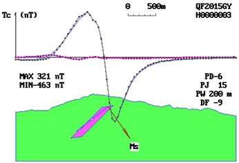
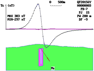
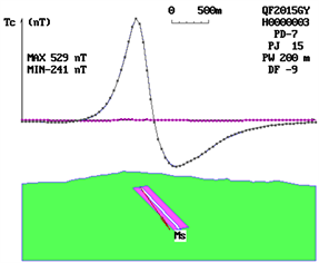
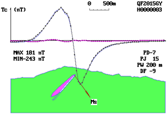

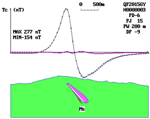
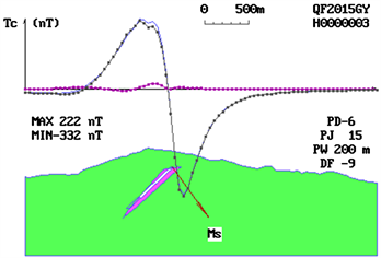
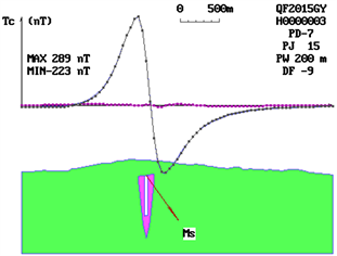
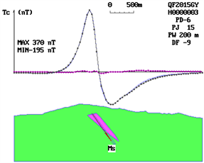
Figure 2. Symbolic recognition of three types of magnetic source morphology under mountain topography.
plate strike of the magnetic source is changed respectively, in order to explain the best fitting between the anomaly and the unknown anomaly, and finally determine the spatial shape of the magnetic source.
3. Method and Technology
3.1. Three Steps to Determine the Shape of an Unknown Magnetic Source
1) The unknown anomaly was explained by the triangular plate interpretation method, and the identification parameters were obtained preliminarily. All the parameters except the thickness in the result were interpreted by the book board method, combined with the thickness of 3 to 5 times, the thick plate model and the pinnacle model were calculated. Three abnormal profile curves of lens model. Three identification parameters are obtained by using the method of log plate. Comparing with the identification parameters of unknown anomalies, the types of magnetic source morphology of unknown anomalies can be identified.
2) The triangular system interpretation method corresponding to the magnetic source morphology model is used to gradually increase the thickness of the model to explain the anomalies. Each time, the identification parameters and the variation of the remaining anomalies are observed. Under normal conditions, the identification parameters will be gradually close to the direction of “eee”, and the remaining anomalies will be gradually close to the horizontal coordinate axis. When the model thickness is gradually iterated and the western details of the model are adjusted appropriately, the identification parameters will be considered as “eee”. The magnetic source profile in the magnetic anomaly profile can be obtained.
3) Combined with the abnormal plan, the length of the model combination board is adjusted, and the spatial shape of the magnetic source which causes the unknown magnetic anomaly is determined.
3.2. Technical Processing in Inversion Process
1) In the process of adopting progressive iteration of model thickening, it is shown that the thickness of the model is excessive when the identification parameters are found to be reversed. When it is found that the values of the identification parameters cannot trend to “e” at the same time, and the local residual anomalies are obvious, It is shown that the model for interpretation needs to be revised, and the details of the model should be adjusted repeatedly, and the consistency of identification parameters towards “e” and the change of residual anomalies should be observed in order to make the interpretation model close to the true magnetic source shape (Figure 3).
Explanatory text MX Model morphology of magnetic source; JS The explanatory form of Magnetic Source; MS Effective magnetization direction in section; PD The number of bias points of Magnetic Source in the profile; PJ Interpretation profile angle; PW Deviation of interpretation profile and anomaly origin; DF Top angle of the top surface of the magnetic source.
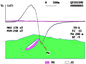
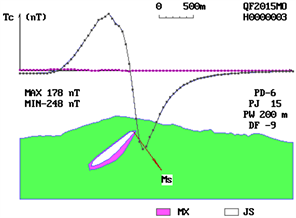
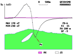
Figure 3. Flow chart of shape determination of field source profile.
2) In order to determine the shape of magnetic source accurately, it is necessary to adopt the combination of first section, later plane, section and plane, step by step iteration and careful adjustment before it can be realized.
4. Application Examples
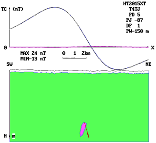
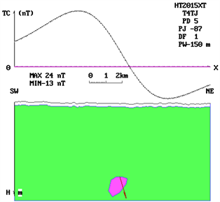
The aeromagnetic anomaly of Begonia, which is provided by electronics in the Academy of Sciences, is inverted into four parts by triangulation. The deep anomaly is identified as “NNP” symbol combination pattern after being explained by the triangular system book plate method. It is considered to be the magnetic source form of “pinnacle type”, and the method of triangulation pinnacle class is used to explain it step by step. According to the position of residual anomaly, the thickness of morphological details is adjusted, and the identification parameters are gradually changed to the symbol mode of “eee”. It is concluded that the profile of the magnetic source is “kernelike” in the upper, larger and lower order. Combined with the progressive iteration of the anomalous plane characteristics, the spatial shape of the magnetic source is finally determined to be a short-axis kernelike. After careful study of the geological and mineral background in the anomalous area, it is inferred that the short-axis kernelike magnetic source should be the magnetic shell of the contact zone between the concealed rock mass and its surrounding rock. The three plate-shaped magnetic bodies in the upper part should be the product of post-magmatic hydrothermal activity and should be related to precious metals and non-ferrous metal blind ore. The identification of the magnetic source form is of great significance to the prospecting in the area. After the shape of the “kernelike” magnetic source profile has been determined, combining with the abnormal plane characteristics, the direction length of the plate forming the “kernelike” has been adjusted step by step, and through progressive iteration, Finally, the spatial shape of the magnetic source is determined to be “short axis kernelike”. After careful study of the geological and mineral background in the anomalous area, it is inferred that the short-axis kernelike magnetic source should be the magnetic shell of the contact zone between the concealed rock mass and its surrounding rock. The three plate-shaped magnetic bodies in the upper part should be the product of post-magmatic hydrothermal activity, which is related to precious metals and non-ferrous metal blind ore to a large extent. The identification of the magnetic source form is of great significance to the prospecting in the area (Figure 4).
 (a)
(a)
 (b)
(b)
 (c)
(c)
Figure 4. Morphological identification and determination of deep magnetic source bodies of Haitang aeromagnetic anomaly. (a) The “NNP” formula is obtained by using the inversion of the plate method, and the magnetic source is identified as a “pinnacle” magnetic source; (b) The “NNP” formula is still obtained by using the method of pinnacle interpretation, which indicates that the thickness of the pinnacle needs to be increased; (c) By adjusting the thickness and the detail of the pinnacle, the identification parameters are changed to the formula of “eee” and the shape is determined to be “kernel”.
5. Conclusions
The problem of magnetic source shape determination is simplified into iterative inversion of magnetic source thickening and detail adjustment after symbol recognition.
The trigonometric interpretation method with the function of differential and integral not only gives the space position, occurrence, size, magnetic characteristics and intensity of the magnetic source, but also the identification parameters of unknown curves can be determined according to the calculus in applied mathematics. Under the premise that the magnetic source can be considered as homogeneous magnetization, the spatial shape of the magnetic source can be determined by the adjustment of the gradual thickness and the detail.
In this paper, a unified expression of multi-class magnetic sources combined with variable size and uniform multi-plate is given, which is an infinite number of interpretation methods corresponding to the variable model for the triangle system, which is helpful to the detailed study of the morphology of the hidden magnetic source.
Cite this paper
Cai, J.X. (2018) Differential Integrals of Curves and Inversion of Magnetic Source Morphology. Journal of Applied Mathematics and Physics, 6, 1160-1169. https://doi.org/10.4236/jamp.2018.66098
References
- 1. Cai, J.X. (1989) Magnetic Anomaly Triangle Interpretation System. Geological Publishing House, 12-21.
- 2. Cai, J.X., Li, Y. and Dai, Q.W. (2016) Research on the Source of Magnetic Anomaly Field. China Science and Technology Paper Online.
- 3. Yan, Y.P., Dai, Q.W. and Cai, J.X. (2014) Theory and Method of Conjugate Interpretation of Magnetic Anomalies. Geological Publishing House, 89-91.
- 4. Brain, D.A., Bagenal, F. and Acuna, M. (2000) Magnetic Morphology from MGS MAG. Bulletin of the American Astronomical Society, Summary.
- 5. Grant, F.S. (1965) Gravity and Magnetic Methods, the Quantitative Interpretation of Magnetic Anomalies. Interpretation Theory in Applied Geophys, 340-350.
- 6. Liu, X.Z. (1993) Principle and Application of spectral Analysis of Gravity and Magnetic Anomalies. Chongqing Publishing House, Chongqing, 132-167.
- 7. Yan, Y.P., Dai, Q.W., Cai, J.X. and Lu, G.M. (2011) Magnetic Anomaly Conjugate Element Inverse Interpretation Method. Journal of Central South University, Natural Science Edition, 731-737.
- 8. Cai, J.X. (1990) A Method of Magnetic Anomaly Inversion and Distortion Correction. Collection of Computational Geophysical Studies. Earthquake Press, 279-288.