Open Journal of Soil Science
Vol.4 No.3(2014), Article ID:43617,11 pages DOI:10.4236/ojss.2014.43012
Bowen Ratio Energy Balance Measurement of Carbon Dioxide (CO2) Fluxes of No-Till and Conventional Tillage Agriculture in Lesotho
Deb O’Dell1*, Thomas J. Sauer2, Bruce B. Hicks3, Dayton M. Lambert4, David R. Smith1, Wendy Bruns1, August Basson5, Makoala V. Marake6, Forbes Walker1, Michael D. Wilcox Jr.7, Neal Samuel Eash1
1Institute of Agriculture, University of Tennessee, Knoxville, USA
2United States Department of Agriculture (USDA) Agriculture Research Service (ARS), Ames, USA
3MetCorps, Norris, USA
4Department of Agricultural & Resource Economics, University of Tennessee, Knoxville, USA
5KEL Growing Nations Trust, Mohaleshoek, Lesotho
6Department of Soil Science & Resource Conservation, National University of Lesotho, Maseru, Lesotho
7Purdue University, West Lafayette, USA
Email: *dodell3@utk.edu
Copyright © 2014 by authors and Scientific Research Publishing Inc.
This work is licensed under the Creative Commons Attribution International License (CC BY).
http://creativecommons.org/licenses/by/4.0/


Received 14 January 2014; revised 14 February 2014; accepted 21 February 2014
Abstract
Global food demand requires that soils be used intensively for agriculture, but how these soils are managed greatly impacts soil fluxes of carbon dioxide (CO2). Soil management practices can cause carbon to be either sequestered or emitted, with corresponding uncertain influence on atmospheric CO2 concentrations. The situation is further complicated by the lack of CO2 flux measurements for African subsistence farms. For widespread application in remote areas, a simple experimental methodology is desired. As a first step, the present study investigated the use of Bowen Ratio Energy Balance (BREB) instrumentation to measure the energy balance and CO2 fluxes of two contrasting crop management systems, till and no-till, in the lowlands within the mountains of Lesotho. Two BREB micrometeorological systems were established on 100-m by 100-m sites, both planted with maize (Zea mays) but under either conventional (plow, disk-disk) or no-till soil management systems. The results demonstrate that with careful maintenance of the instruments by appropriately trained local personnel, the BREB approach offers substantial benefits in measuring real time changes in agroecosystem CO2 flux. The periods where the two treatments could be compared indicated greater CO2 sequestration over the no-till treatments during both the growing and non-growing seasons.
Keywords:CO2 Flux; CO2 Emissions; Soil; Soil Carbon; Tillage; Till; No-Till; Bowen Ratio; Micrometeorology; Agriculture; Climate Change; Lesotho; Africa

1. Introduction
Although some aspects of climate change arguments remain contentious, there is general scientific acceptance of the conclusion of the Intergovernmental Panel on Climate Change (IPCC) that increases in atmospheric concentration of carbon dioxide (CO2) and other greenhouse gasses (GHGs) have contributed to increases in global temperatures and associated climate change. The IPCC report summarized the extent and cause of this increase, noting that human activities have increased atmospheric CO2 by approximately 40 percent since the mid-1700s [1] . While most anthropogenic CO2 emissions result from fossil fuel combustion, the US Council for Agricultural Science and Technology (CAST) Task Force Report stated that agriculture produces 13.5 percent of GHG emissions world-wide [2] . According to Denef et al. [3] CO2 emissions from agriculture in the US result primarily from practices that reduce the amount of organic carbon in the soil, e.g., fallow or intensive tillage. After the lithosphere and oceans, soil organic matter represents the earth’s third largest pool of carbon (C), greater than the C pools in the atmosphere and biosphere [4] . An increasing amount (presently ~12 percent, see Wood et al. [5] ) of the world’s land area is used for food production. The CAST Task Force reports that modified agricultural practices could help reduce agricultural CO2 emissions. The United Nations Food and Agriculture Submission to the United Nations Framework Convention on Climate Change (UNFCCC) supports this view, stating that agriculture has the potential to contribute to the mitigation and stabilization of the concentration of atmospheric GHGs by promoting the use of agricultural management practices that enhance C sequestration in soils while discouraging the use of agricultural practices that promote the emission of CO2 from soil to the atmosphere [6] . At the same time, such practices would increase the amount of carbon in soils, to the benefit of plant growth.
Converting from tillage to no-till (NT) as an agricultural management practice has been identified as having potential to reduce CO2 emissions [7] -[9] . Tillage-induced disturbance increases aeration within the top soil horizons, which fuels microbial decomposition of organic matter, increasing soil respiration and CO2 emissions [10] . West and Post [9] found in their meta-analysis of 67 different long-term (greater than five years) studies that a change from conventional tillage to NT generally produced a significant increase in soil organic carbon (SOC) in the top 7-cm of soil in all experiments except under a rotation of wheat followed by fallow treatment [9] .
However, the potential of NT to increase soil C has been contested [11] -[13] , especially for moist, cool climates and for heavy, textured soil [14] . Many studies have found that soil samples deeper in the profile do not show the effects of different tillage practices affecting shallower soil layers. Clearly, more research is needed to provide data on the value of NT as an agricultural practice in specific climates and soil types.
Measuring soil C is fundamental to understanding sequestration rates and amounts in soils managed under contrasting tillage regimes. Under high intensity tillage, C can be lost in a relatively short amount of time whereas NT systems sequester C but at very low rates with estimates ranging from 97 kg C ha-1 yr-1 in a dry climate after 20 years [15] to the mean rate of 480 kg C ha-1 yr-1 that West and Post found from long-term experiments in various climates around the globe [9] . It is critical to measure the impact of tillage, because it has been implicated as the key contributor to CO2 emissions from soil.
Due to the slow rate of C sequestration and spatial variation in many soils, annual changes in soil C are small and can be difficult to quantify. Interannual climactic variability also impacts carbon emissions from soils and soil carbon measurement over time. The Food and Agriculture Organization of the United Nations (FAO) submission to the UNFCCC [6] [16] summarized the challenges in measuring the capacity of agricultural practices and soil to sequester or emit C. These challenges entail variability in soil type and C content within a field; the need to measure small year-to-year changes in soil C; and previous land use practices. There is presently insufficient understanding to warrant confident assessment, or even to design definitive field studies, particularly for developing countries. Even though the C content of agricultural soils increases slowly, can be reversed, and can only play a minor role in comparison with the CO2 emissions of fossil fuels, Smith [17] suggests that concerted efforts to reduce agricultural CO2 emissions—including enhanced soil carbon sequestration—will be required to achieve desired global reductions in emissions.
Developing countries in sub-Saharan Africa represent a region where conservation agriculture (CA) practices improve soil quality as well as stabilize or increase yield while reducing C emissions. In brief, the FAO describes CA as a farming system that prescribes minimal soil disturbance such as no tillage, maintains organic cover on the soil surface and crop rotations [18] . As much as three-quarters of the agricultural land in sub-Saharan Africa has been degraded by erosion and depletion of soil nutrients [19] -[21] . The Kingdom of Lesotho in particular is said to have the highest rate of soil erosion in both central and southern Africa [22] . Consequently Lesotho has declined from a net grain exporter in the 1800s [23] to producing less than 30 percent of its own national grain demand in the present day [24] . Increasing soil organic C using CA could improve agricultural production and ecosystem protection by enhancing soil fertility, water holding capacity, aggregate stability and water infiltration [25] .
Since C emissions from land are variable and occur in minute quantities over large scales, they are hard to quantify with confidence. There are two main approaches for measuring CO2 exchange over agricultural ecosystems including the use of static chambers and micrometeorological techniques [2] . The two primary micrometeorological methods are the Bowen Ratio Energy Balance (BREB) system and eddy covariance. Of these two, the latter requires much more complex instrumentation, and usually requires more expert on-site technical attention than the former. Dugas [26] compared three BREB systems with nine soil chambers and found good CO2 flux agreement between the two methods. He also noted that the BREB method integrates the soil-atmospheric boundary layer interactions over a much larger area than the chamber method and thus accommodates more of the spatial variability of CO2 flux from soil, allowing high resolution measurements representative of larger expanses. Since there are substantial temporal, spatial, and maintenance challenges in using chamber systems, the BREB approach has been favored for present use. The study reported here is viewed as a field test of the BREB approach, conducted in demanding circumstances in a very mountainous area.
The present study was designed to test the hypothesis that there are no significant differences between longterm net emissions of CO2 over an area of conventional tillage (Till) and an otherwise similar NT area typical of traditional small scale farming methods in Lesotho. The study compared CO2 flux between Till and NT treatments over an eighteen month period.
2. Materials and Methods
2.1. Site Description
BREB measurements of soil and micrometeorological properties were collected from December 2010 to June 2012 in Maphutseng (30˚12.828'S, 27˚29.747'E for the Till plot and 30˚12.788'S, 27˚29.718'E for the NT, 1457 m elevation) in the district of Mohale’s Hoek in southern Lesotho [27] . The study site was located in the Maphutseng river valley on the first terrace above the alluvial floodplain. The study site is in a very mountainous region, but is delineated as the southern lowlands of Lesotho.
Approximately 85 percent of the annual rainfall occurs during the warm season months, from October through March/April. Annual precipitation in the district of Mohale’s Hoek averages less than 700 mm yr−1 [28] . Snow and rain occur during the cold season between May and July. Extreme weather conditions such as high winds and hail can occur throughout the year.
The soil was classified as the Phechela series (fine, montmorillonitic, mesic Typic Pelludert); the site was level, with a slope not exceeding 2 percent. While the site classifies as a udic soil moisture regime, there are significant dry periods after crop harvest and through the winter months.
Two adjacent one ha fields were selected for the experimental plots. The NT plot was untilled pasture for almost 30 years until 2008 prior to the start of the present study while the Till plot was kept in sustained tillage over the same period, with a minimal number of non-crop years. The average pH for four soil samples taken February 24, 2011, of the top five cm and 5 - 10 cm depth of soil for the NT plot was 6.83, while the pH of the top 0 - 5 cm and 5 - 10 cm averaged 6.87 and 6.85 respectively in the Till plot (1:1 soil:water ratio) [29] . The bulk density for the Till plot was measured in July 2012 at 1.21 and 1.23 g/cm3 for 0 - 5 cm and 5 - 10 cm depths respectively. The bulk density for the NT plot, measured in August 2013 was 1.10 and 1.13 g/cm3 for 0 - 5 cm and 5 - 10 cm depths respectively. The average yield for the Till and NT plots during the 2012/2013 planting and harvest season was not significantly different at 7.02 and 6.59 tonnes/ha respectively and the plots were under similar cropping management throughout the experiment.
The NT field was seeded with maize (Zea mays L.) using a 2-row VenceTudo Planter in November 2011. The Till field was prepared with conventional tillage methods using a moldboard plow with two cultivation passes using a tandem disk before planting maize with a 2-row VenceTudo Planter in November of 2011. Interrow spacing was 90 cm for both plots with population densities seeded at approximately 29,600 plants ha−1 [27] .
2.2. Micrometeorological Measurements
Soil and atmospheric properties were measured and recorded using a BREB system following the theory and experimental procedures laid out by Dugas [26] . The one ha size of the plots and the vegetation and topography surrounding the plots provided a sufficient uniform measurement area (fetch) for micrometeorology measurements. A BREB micrometerological station was built for each plot, with a rotating arm center-mounted on an aluminum mast for height adjustment above the canopy and anchored by a tripod, as shown in Figure 1. The arm rotated on a shaft powered by a 12 V DC electric gearmotor (model 4Z834, Dayton), until it came to rest in a near-vertical position. A horizontal shielded air intake was mounted at both ends of the arm, approximately 1.5 m apart. Each air intake housed humidity and temperature sensors and CO2 intake tubes for measurements at two heights (adjusted routinely so as to be 0.2 and 1.7 m above the top of the growing maize canopy). Air temperatures were measured using thermistors (designed and supplied by TJ Sauer). Water vapor pressure was calculated from hygroclip humidity and temperature probe data (model HC2-S3-L; Rotronic, Switzerland supplied by Campbell Scientific, Inc, Logan, UT). Fans drew air into the intakes, providing a constant flow of ambient air over the sensors at 0.34 m3/min. Carbon dioxide concentrations were measured with an absolute, non-dispersive infrared (NDIR) gas analyzer (model LI-820, LI-COR Inc., Lincoln, Nebraska, USA). Air intake openings faced in the direction of the most prevalent winds (near North).
Net radiation was measured with a net radiometer (model Q-7.1, Radiation Energy Balance Systems (REBS), Seattle, WA) that was attached to the mast at a height of 2 m. A soil heat flux plate (model HFT3, REBS) at a depth of 0.06 m was used to measure soil heat flux. Soil temperature was measured with two Type “T” thermocouples buried at 0.02 m and 0.04 m. Barometric pressure was measured using a silicon pressure sensor (model SB-100, Apogee, Logan, UT). A three-cup anemometer (model 014A, Met One Instruments, Inc., Grants Pass, OR) was installed at each BREB location at a height of 5 m to measure wind speed and a recording rain gauge
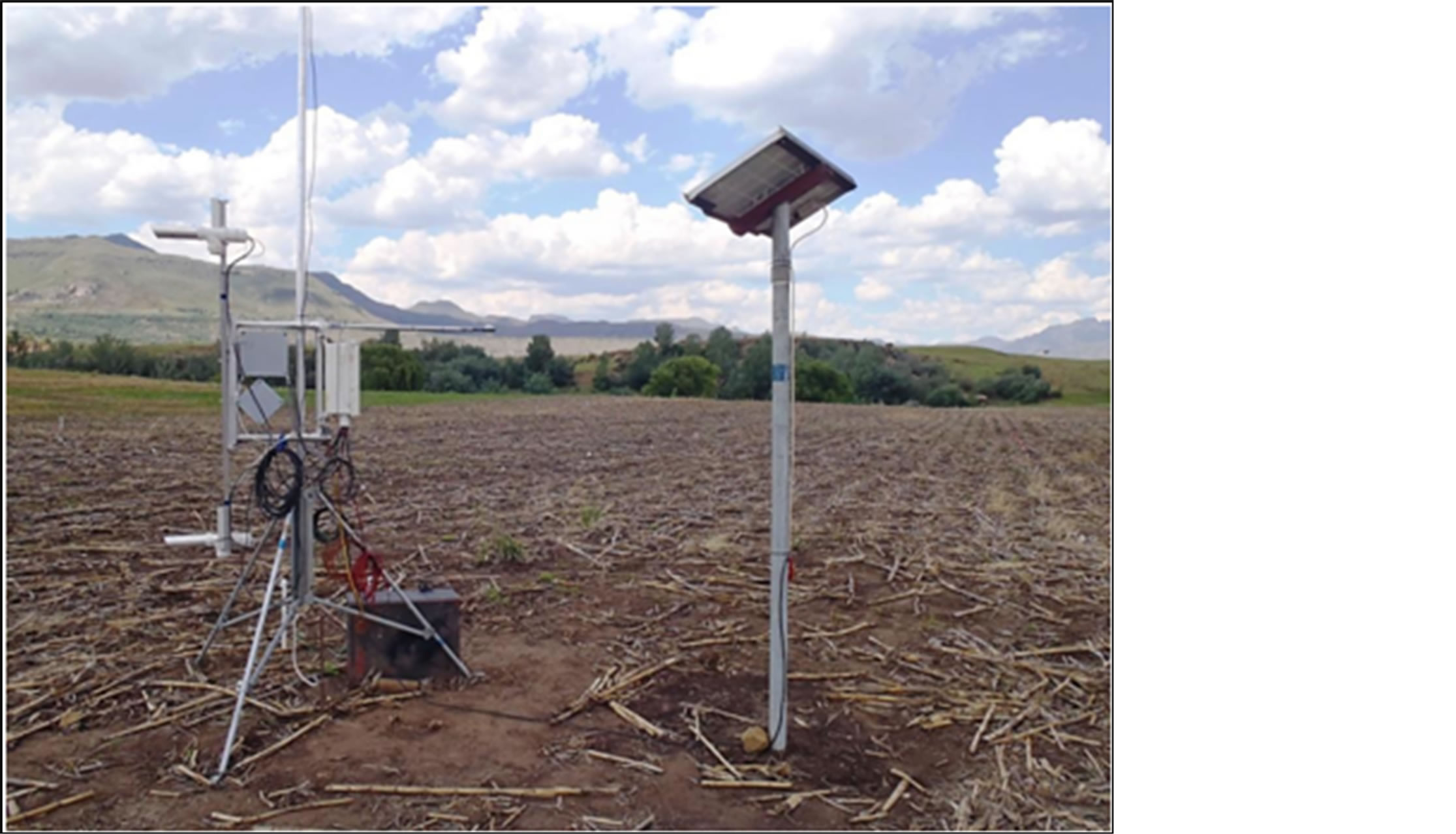
Figure 1. Photograph of micrometeorological station in Maphutseng.
(model TE525, Campbell Scientific Inc.) was installed nearby.
A data logger (Model CR23X, Campbell Scientific Inc.) read sensor data every five seconds. After arm rotation there was a time delay of seven seconds to allow for gas to be purged from the tubing. The data logger computed and stored 5-min averages of these readings. After each 5 min average was stored, the data logger prompted the rotation of the arm swapping the lower and upper positions of the air intakes inlets that housed the temperature and humidity sensors. Moving the sensor arms allowed each sensor to measure the two positions thereby cancelling accuracy issues with each sensor and provided the precision necessary to derive accurate measurements of differences in temperature, humidity and CO2 concentration between the two heights. Two 70 W solar panels and three 12 V batteries wired in parallel powered each BREB unit.
Soil samples were collected to measure soil organic carbon concentrations towards the beginning of BREB measurements on February 4, 2011 for the NT field and February 24, 2011 for the Till field. Total organic C concentration was determined by dry combustion at 900C (VarioMax CNS macro elemental analyzer, Elementar, Hanau, Germany).
2.3. Data Analysis
The following equations were used to calculate the Bowen ratio and the CO2 flux density based on research developing and refining the BREB approach [26] [30] -[36] in a protocol assembled by Dr. T.J. Sauer (personal communication, 2011). Five-min temperature and water vapor differences were averaged at 30-min intervals to calculate the Bowen ratio (b):
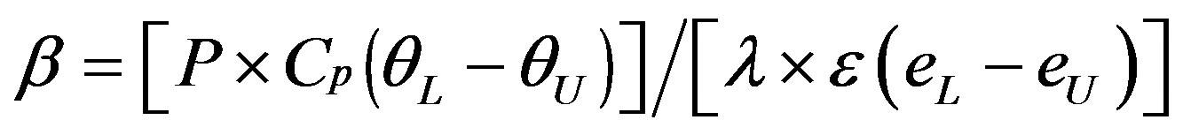 (1)
(1)
where P is the atmospheric pressure in kPa (measured), Cp is the specific heat capacity of air at constant pressure (1004.67 J∙kg−1∙K−1), qL and qU are the potential temperatures at the lower (L) and upper (U) positions (K), l is the latent heat of vaporization of water (2.45 × 10⁶ J∙kg−1), e is the ratio of the molecular weights of air and water (0.622), and eL and eU are the vapor pressures at the lower and upper positions (kPa) [30] -[33] [35] .
Potential temperature, q, was calculated from the thermistor air temperature data:
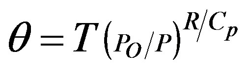 (2)
(2)
where T is the thermistor temperature (measured in ˚C and converted to K, i.e., K = ˚C + 273.16), PO is the standard reference pressure (100 kPa), P is the observed pressure, and R is the gas constant (8.314 J∙K−1∙mol−1) and Cp is the specific heat capacity of air (~29.1 J∙mol−1∙K−1) [35] .
Latent heat flux density, LE (W∙m−2) was calculated as:
 (3)
(3)
where Rn is the measured net radiation (W∙m−2) and G0 the soil heat flux at the soil surface (W∙m−2) [26] [31] -[34] . Since soil heat flux was measured with flux plates at a depth of 0.06 m below the surface, measured soil heat flux values were corrected for heat storage in the 0 - 0.06 m soil layer (i.e.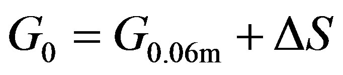 ).
).
 (4)
(4)
where DS is the change in heat storage above the soil heat flux plate (W∙m−2), C is the volumetric heat capacity of the soil (MJ∙m−3∙K−1), DT is the change in temperature (current minus previous) of the soil above the heat flux plate (K) taken from average soil temperature measurements at 0.02-m and 0.04-m depths, Dt is the time step (s), z is the depth of the flux plate (0.06 m) and 1 × 10⁶ converts from MJ to J. The volumetric heat capacity (C) is calculated for each time step.
Sensible heat flux density, H (W∙m−2) was calculated as [26] [33] [35] :
 (5)
(5)
The sign conventions used for this study are that Rn is positive when energy is moving down toward the soil surface, H and LE are positive when moving up and away from the surface, and G is positive when moving down from the top of the soil surface [26] [34] .
Turbulent diffusivity for sensible heat, Kh (m2∙s−1) was calculated as:
 (6)
(6)
where raCp is the volumetric heat capacity for air (1200 J∙m−3∙K−1), Dz is the sensor separation distance (1.5 m) [35] .
A, the CO2 flux density (kg∙m−2∙s−1) was calculated as:
 (7)
(7)
where Kc is the turbulent diffusivity for CO2 (m2∙s−1) which is assumed to be equal to the turbulent diffusivity for sensible heat (Kh), and Drc is the average difference in CO2 density between measurement heights converted from the LI-820 CO2 concentration output of ppm to kg CO2 m−3 [26] [32] [33] . The sign convention for CO2 flux is that an upward flux is positive and a downward flux is negative.
The CO2 flux was corrected for temperature and vapor density differences at the two measurement heights using the following equation:
 (8)
(8)
where Acorr and A are in kg∙m−2∙s−1, rc is the average CO2 density at both measurement heights (g∙m−3), ra is the density of dry air (~1200 g∙m−3) [36] . The CO2 flux density presented in this paper follows customary sign conventions where a positive Acorr number represent CO2 emissions from the soil and a negative Acorr represents C sequestration [26] .
Based on research examining conditions where the BREB method fails [34] , raw data were rejected that came within the range of the thermistor sensors’ resolution, which was: |Thermistor DT| < 0.02˚C.While the sensor resolution range for vapor pressure was 0.01 kPa, over one third of the vapor pressure differences, De, fell within that range, so raw data was rejected within the range of |De| < 0.004 kPa. These data were removed and replaced by values computed by linear interpolation [34] .
Similarly, because of the Bowen ratio definition using measured vertical temperature and humidity differences, computed CO2 fluxes are subject to large error as the ratio approaches −1, which frequently occurs near sunrise, sunset, or during rainfall [34] [37] . In recognition of this, values of the Bowen ratio in the range −0.95 < b < −1.05 were replaced via linear interpolation. Data collected during precipitation events were omitted because of the questionable performance of Rn and G sensors during and immediately after rainfall. Graphs of both 5-min and 30-min averaged raw data and calculated energy fluxes were visually inspected to detect problems with sensors.
3. Results and Discussion
The BREB system as used here provides redundancy for some sensors to allow data collection when instruments stopped working. For example when the net radiometer on the Till unit malfunctioned (due to birds pecking a hole in the dome), the sensor values on the NT unit were used. When thermistor temperature data were not available for analysis, the ambient air temperatures recorded by the Rotronic HC2-S3 humidity and temperature probe at the two heights were used. However, the HC2-S3 sensors are more slowly responsive than the thermostors, which affect the calculations. This also meant that to calculate flux for the Till instrument, the NT net radiometer had to be working. DS calculations were made with the average of the top two thermocouples at 0.02- m and 0.04-m depth below the surface, so a malfunction of the lower soil thermocouples on the Till unit necessitated reliance on the top soil thermocouple during the period of malfunction.
Due to sensor and data collection issues, there was not sufficient data to provide conclusive comparisons between the two treatments, however, some data are available for analysis. Data from one five-day period that could be viewed as being representative of the non-growing season are presented in Figures 2 and 3. These figures show the energy balance for both NT and Till treatments during a 5.5 day period starting at 12 noon on August 29th through September 3rd 2011 (Decimal Day of Year (DOY) 241-247), about 2 months before crops were planted. The abscissa is ordered according to local time (two hours ahead of GMT). The graphs of the energy balance (Figures 2 and 3) show similar trends between the two treatments, though the No-Till shows shorter and wider peaks of sensible heat than the Till, which would be consistent with greater absorption capacity of the denser organic residue on the NT surface.
A graph of the CO2 flux density for this period is shown in Figure 4. Combined with two additional days in September, 2011, the average CO2 flux density for seven days between DOY 242 and 250 was −0.104 and −0.033 g∙m−2∙hr−1 for the NT and Till plots respectively. A standard t-test results in the conclusion that the
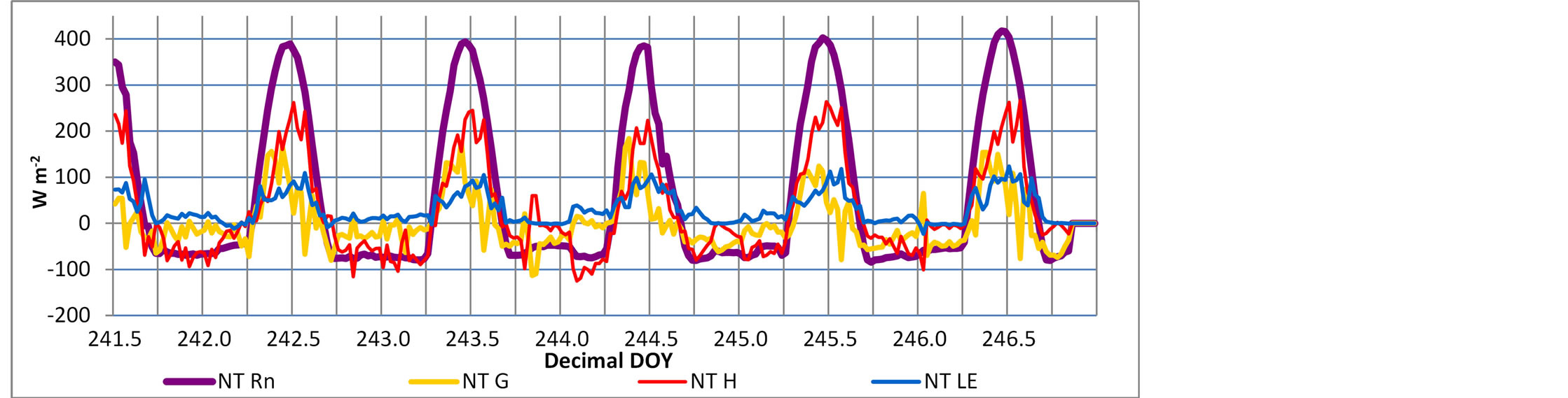
Figure 2. Energy balance for NT treatment at Maphutseng from August 29 through September 3.
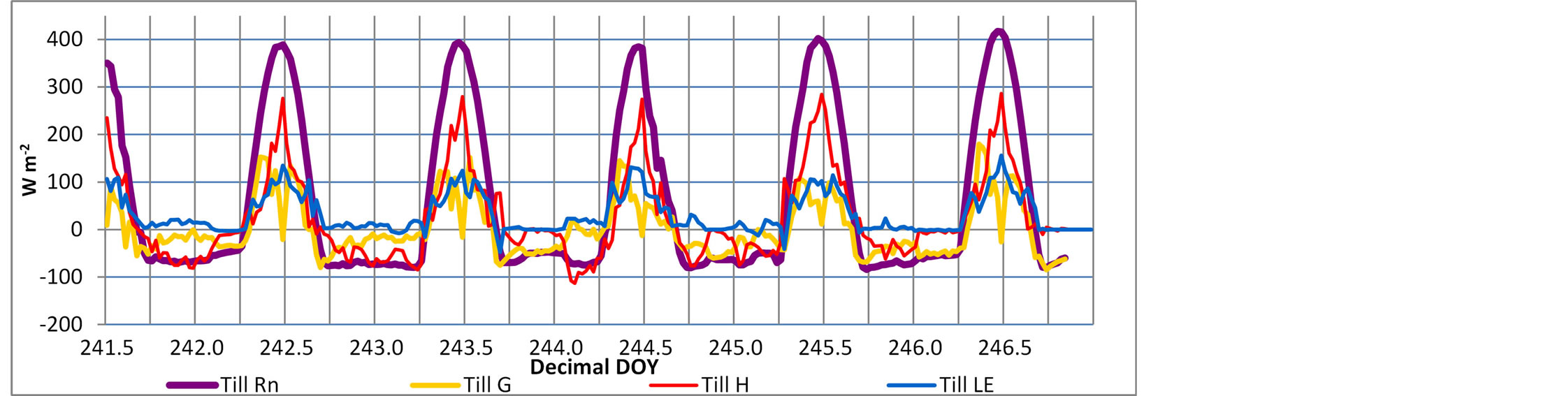
Figure 3. Energy balance for Till treatment at Maphutseng from August 29 through September 3.
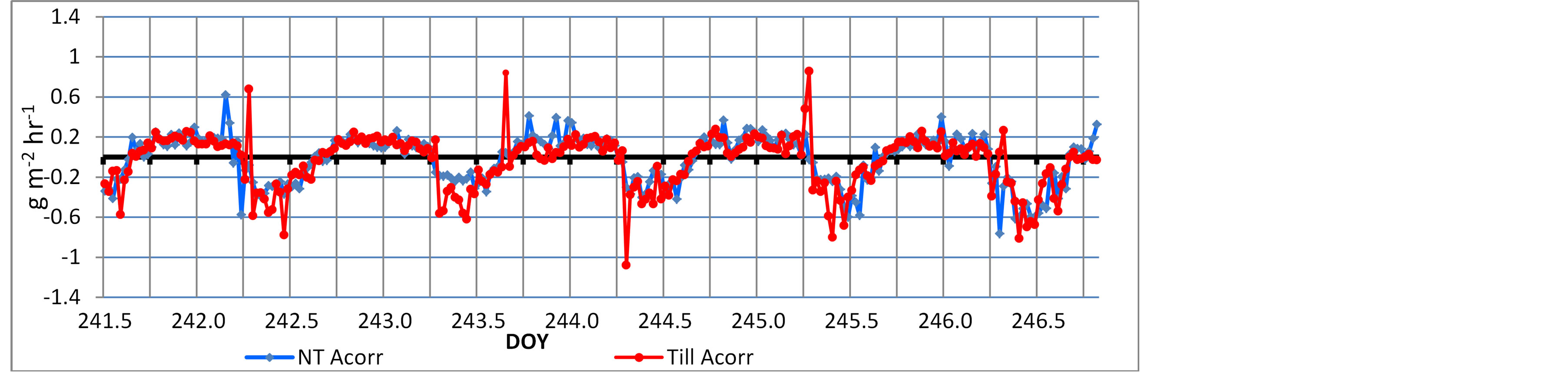
Figure 4. CO2 flux density for NT and Till plots for DOY 241-247 (August 29- September 3, 2011).
average fluxes were significantly different for the last two days in September, but there was no significant difference for the first 5 days shown in the graph (alpha = 0.10). Cumulative values of CO2 for these seven days total −17.4 and −5.47 g∙m−2 indicating greater C sequestration by the NT plot.
The CO2 flux was calculated for one period during the growing season in January 2012 as shown in Figure 5 . Extreme CO2 flux values (less than −4 g∙m−2∙hr−1 and greater than 4 g∙m−2∙hr−1) were considered erroneous and were removed and interpolated. These values occurred most often at sunrise and sunset or when the temperature gradient was opposite in sign from the vapor pressure gradient [36] . Twenty-nine percent of the Till data for this period and twenty percent of the NT data were removed and interpolated. The interpolated average CO2 flux densities for this period are −1.11 and −0.22 g∙m−2∙hr−1 for the NT and Till plots respectively and result in cumulative values of −106.49 and −21.47 g∙m−2 for the NT and Till plots respectively. A contributing factor to reduced data collection during the growing season was rainfall, which is a reason to reject raw data for BREB calculations [34] [37] .
During this period daytime temperatures reached 37˚C with nighttime temperatures reaching a low of 12˚C. Sensible heat fluxes were greater than in the non-growing (August and September) season represented in Figure 4. This difference and the presence of a rapidly growing crop explain in part the greater CO2 fluxes during this later period (January). For the growing season data set, the mean difference in flux was statistically significant
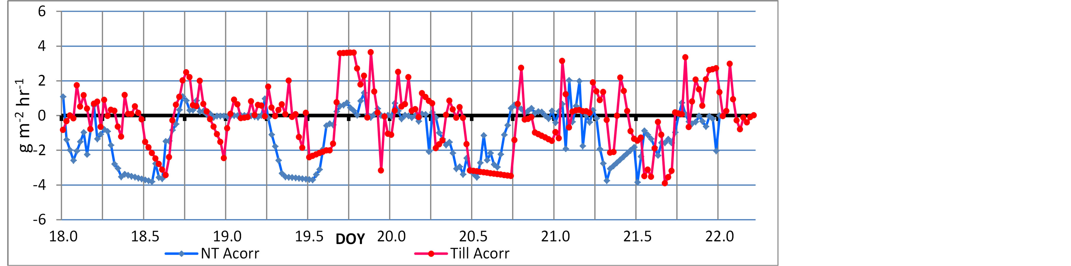
Figure 5. CO2 flux density for NT and Till plots during growing season.
(alpha = 0.05).
It was postulated that the spikes that occurred with increased frequency in the growing season data likely resulted from the use of air temperature readings from the Rotronic humidity and temperature probe. Reliance on these sensors was necessitated by the failure of some of the thermistor sensors. Figure 6 is a graph of both the thermistor sensors (shown in purple) and Rotronic (shown in green) 5-min readings for both the Till and NT instruments, where the right (R) temperature (T) sensor exchanges positions every 5 minutes with the left (L) sensor between the upper and lower heights. Figure 6 does not indicate an obvious difference between the observed 5-min thermistor and Rotronic temperature readings of 8 sensors tracking in the same pattern within 1˚C - 4˚C of each other. However when subtracting the upper sensor reading from the lower to determine the gradient as shown in Figure 7 the thermistor sensors have a distinctly larger difference. Because the difference in potential temperature between the two measurement heights is used in the denominator when calculating the turbulent diffusivity, the smaller the difference, the larger the turbulent diffusivity, which directly affects the calculations of CO2 flux. Near sunrise and sunset, in particular, the sensible heat flux changes sign while the evaporative flux typically reduces but does not reverse in sign (unless dewfall occurs). In these situations, small temperature differences can occur while turbulent exchange remains strong. However, the small gradients of temperature and humidity cause enhanced susceptibility to small errors of measurement, particularly in the Bowen ratio calculations.
The consistent difference between the temperature gradients derived from the two systems (thermistor and Rotronic) is attributed to the substantial differences in the response time of the two sensor systems. To address this issue and to achieve a more accurate reading of temperature and other meteorological data at each sensor height, it has been proposed that after the arms rotate, a delay of one to two minutes be added before collecting five-second readings to allow for the sensors to equilibrate to the new sensor height and atmospheric conditions. This would eliminate vestiges of temperature and vapor pressure properties from the previous position and provide a more accurate and likely stronger difference between the two measurement heights increasing the signal associated with the gradient.
Soil samples were taken at the beginning of the study to provide input into the site characterization. Table 1 shows mean organic C concentrations in the 0 - 5 cm layer and 5 - 10 cm of soil for 16 samples with four samples taken in the top five cm and four between 5 and 10 cm in the NT and Till plots at the start of measurements.
4. Conclusions
Though the BREB system requires expertise and a careful balance of interrelated parts it was still viewed as a preferred choice for remote sites and small fields in Africa as it requires a smaller uniform measurement area and less sophisticated and expensive sensors as compared to eddy covariance. Rotation of sensor arm positions to overcome intrinsic sensor bias was determined to be critical for measuring the temperature and vapor pressure gradient for calculating the energy balance and CO2 flux density for the BREB system.
Implementing the BREB system revealed many challenges in establishing robust instrumentation in a remote setting to satisfactorily capture relevant data. With the experience gained refining the instrument structure and resilience, and analysis of data and meteorological conditions, the BREB approach has a lot of potential in capturing real time exchange of CO2, moisture and temperature, all important aspects for agriculture and climate interactions. More research is needed to determine which processes need finer tuning and which processes provide key information for measuring CO2 flux. Due to the intricacies associated with this type of instrumentation
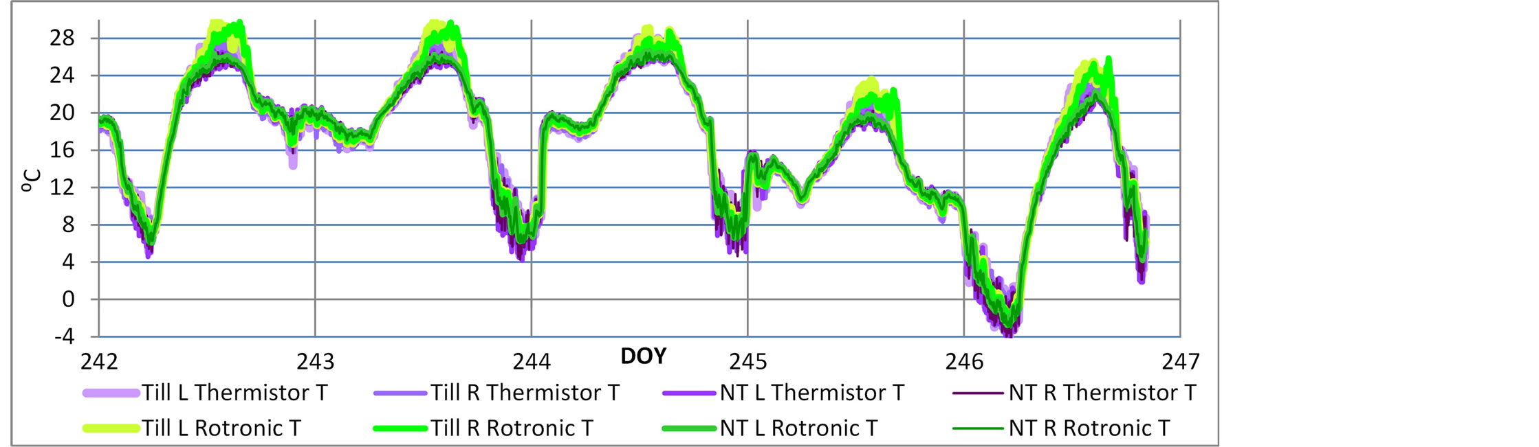
Figure 6. Five-min temperature readings for DOY 241-247 (August 29-September 3, 2011) (thermistor and Rotronic).
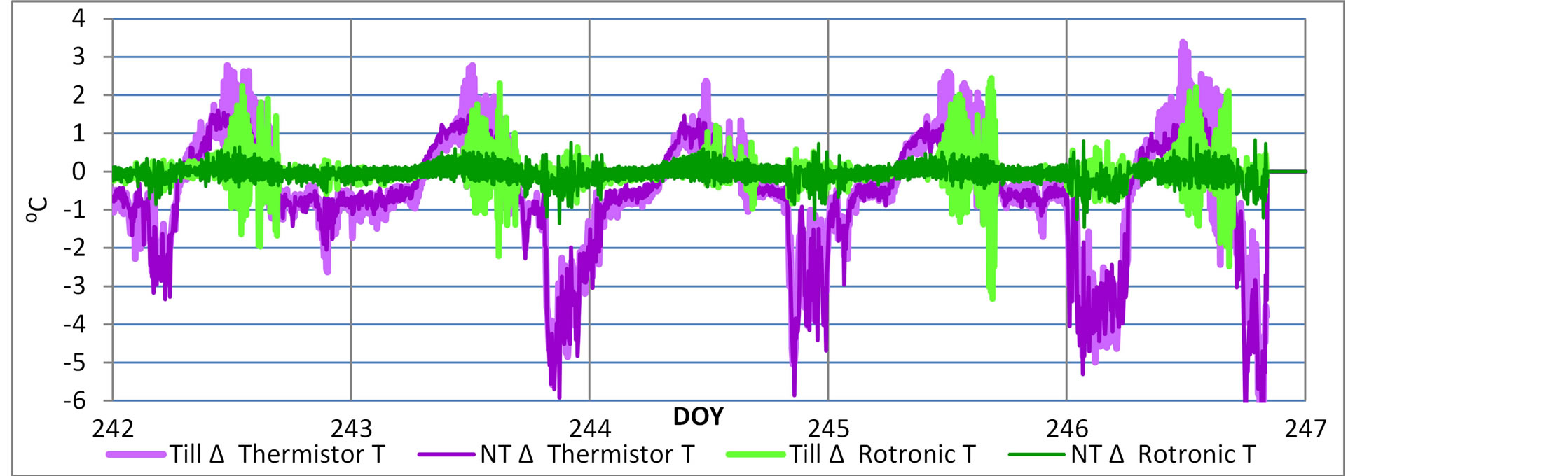
Figure 7. Temperature differences for DOY 241-247 (August 29-September 3, 2011) (thermistor and Rotronic).

Table 1. Organic C concentrations in top 5 cm and between 5 - 10 cm of soil measured at beginning of study.
it is mandatory that on-site personnel have significant interest in the project and in the details of data collection. While this research is difficult, time consuming, and meticulous it is important to understand soil C sequestration and emission issues that could become important if C trading and crediting policies are implemented.
Despite the limitations presented by operating micrometeorological instruments in a remote area of Africa, the data collected indicate that no-till management practices can sequester more carbon than conventional tillage on small-holder farms in Africa.
Acknowledgements
This study was supported by a grant from the Sustainable Agriculture and Natural Resource Management Collaborative Research Support Program (SANREM CRSP) sponsored by the U.S. Agency for International Development’s Bureau of Food Security and the University of Tennessee. The authors also gratefully acknowledge the southern Africa non-profit organization, Growing Nations, for the experimental site in Lesotho, and the USDA Agricultural Research Service for their technical support.
References
- Stocker, T.F., Qin, D., Plattner, G.-K., Tignor, M., Allen, S.K., Boschung, J., Nauels, A., Xia, Y., Bex, V. and Midgley, P.M. (2013) IPCC, 2013: Summary for Policymakers. In: Climate Change 2013: The Physical Science Basis. Contribution of Working Group I to the Fifth Assessment Report of the Intergovernmental Panel on Climate Change. Cambridge University Press, Cambridge and New York.
- Follett, R., Mooney, S., Morgan, J., Paustian, K., Allen Jr., L.H., Archibeque, S., Baker, J.M., Del Grosso, S.J., Derner, J., Dijkstra, F., Franzluebbers, A.J., Janzen, H., Kurkalova, L.A., McCarl, B.A., Ogle, S., Parton, W.J., Peterson, J.M., Rice, C.W. and Robertson, G.P. (2011) Carbon Sequestration and Greenhouse Gas Fluxes in Agriculture: Challenges And Opportunities. Council for Agricultural Science and Technology (CAST), Ames.
- Denef, K., Archibeque, S. and Paustian, K. (2011) Greenhouse Gas Emissions from US Agriculture and Forestry: A Review of Emission. USDA.
- Houghton, R.A. (2007). Balancing the Global Carbon Budget. Annual Review of Earth and Planetary Sciences, 35, 313-347. http://dx.doi.org/10.1146/annurev.earth.35.031306.140057
- Wood, S., Sebastian, K. and Scherr, S.J. (2000) Pilot Analysis of Global Ecosystems: Agroecosystems. IFPRI, WRI, Washington DC.
- FAO (2009) Enabling Agriculture to Contribute to Climate Change Mitigation. United Nations Framework Convention on Climate Change (UNFCCC), Washington DC.
- Schlesinger, W.H. (1999) Carbon Sequestration in Soils. Science, 284, 2095. http://dx.doi.org/10.1126/science.284.5423.2095
- Halvorson, A.D., Wienhold, B.J. and Black, A.L. (2002) Tillage, Nitrogen, and Cropping System Effects on Soil Carbon Sequestration. Soil Science Society of America Journal, 66, 906-912. http://dx.doi.org/10.2136/sssaj2002.0906
- West, T.O. and Post, W.M. (2002) Soil Organic Carbon Sequestration Rates. Soil Science Society of America Journal, 66, 1930-1946. http://dx.doi.org/10.2136/sssaj2002.1930
- Schlesinger, W.H. and Andrews, J.A. (2000) Soil Respiration and the Global Carbon Cycle. Biogeochemistry, 48, 7-20. http://dx.doi.org/10.1023/A:1006247623877
- Baker, J.M., Ochsner, T.E., Veterea, R.T. and Griffis, T.J. (2007) Tillage and Soil Carbon Sequestration. What Do We Really Know? Agriculture, Ecosystems & Environment, 118, 1-5. http://dx.doi.org/10.1016/j.agee.2006.05.014
- Manley, J., van Kooten, G.C., Moeltner, K. and Johnson, D.W. (2005) Creating Carbon Offsets in Agriculture through No-Till Cultivation: A Meta-Analysis of Costs and Carbon Benefits. Climate Change, 68, 41-65. http://dx.doi.org/10.1007/s10584-005-6010-4
- Powlson, D.S., Whitmore, A.P. and Goulding, K.W.T. (2011) Soil Carbon Sequestration to Mitigate Climate Change: A Critical Re-Examination to Identify the True and the False. European Journal of Soil Science, 62, 42-55. http://dx.doi.org/10.1111/j.1365-2389.2010.01342.x
- Angers, D. and Eriksen-Hamel, N.S. (2008) Full-Inversion Tillage and Organic Carbon Distribution in Soil Profiles: A Meta-Analysis. Soil Science Society of America Journal, 72, 1370-1374. http://dx.doi.org/10.2136/sssaj2007.0342
- Six, J., Ogle, S.M., Conant, R.T., Mosier, A.R. and Paustian, K. (2004) The Potential to Mitigate Global Warming with No-Tillage Management Is Only Realized When Practised in the Long Term. Global Change Biology, 10, 155-160. http://dx.doi.org/10.1111/j.1529-8817.2003.00730.x
- UNFCCC (2013) Land Use, Land-Use Change and Forestry (LULUCF). http://unfccc.int/methods_and_science/lulucf/items/4122.php
- Smith, P. (2004) Carbon Sequestration in Croplands: The Potential in Europe and the Global Context. European Journal of Agronomy, 20, 229-236. http://dx.doi.org/10.1016/j.eja.2003.08.002
- FAO (2013) Conservation Agriculture. http://www.fao.org/ag/ca/
- Bai, Z.G., Dent, D.L., Olsson, L. and Schaepman, M.E. (2008) Global Assessment of Land Degradation. Wageningen: International Soil Reference and Information Centre (ISRIC).
- Bai, Z.G., de Jong, R. and van Lynden, G.W.J. (2010) An Update of GLADA—Global Assessment of Land. ISRIC, Wageningen.
- Henao, J. and Baanante, C.A. (1999) Estimating Rates of Nutrient Depletion in Soils of Agricultural Lands of Africa. International Fertilizer Development Center, Muscle Shoals.
- Chakela, Q. and Stocking, M. (1988) An Improved Methodology for Erosion Hazard Mapping Part II: Application to Lesotho. Geografiska Annaler: Series A, Physical Geography, 70, 181-189. http://dx.doi.org/10.1016/j.eja.2003.08.002
- Eldredge, E.A. (2002) A South African Kingdom: The Pursuit of Security in Nineteenth-Century Lesotho. Vol. 78, Cambridge University Press, Cambridge.
- FAOSTAT (2013). http://faostat3.fao.org/home/index.html
- Falloon, P. and Betts, R. (2010) Climate Impacts on European Agriculture and Water Management in the Context of Adaptation and Mitigation—The Importance of an Integrated Approach. Science of the Total Environment, 408, 5667-5687. http://dx.doi.org/10.1016/j.scitotenv.2009.05.002
- Dugas, W.A. (1993) Micrometeorological and Chamber Measurements of CO2 Flux from Bare Soil. Agricultural and Forest Meteorology, 67, 115-128. http://dx.doi.org/10.1016/0168-1923(93)90053-K
- Bruns, W.A. (2012) Energy Balance and Carbon Dioxide Flux in Conventional and No-Till Maize Fields in Lesotho. Master’s Thesis, University of Tennessee, Knoxville.
- Moeletsi, M.E. (2013) Agroclimatic Characterization of Lesotho for Dryland Maize Production. Master’s Thesis, 2004. http://etd.uovs.ac.za/ETD-db/theses/available/etd-08232005-104915/unrestricted/MOELETSIME.pdf
- Kalra, Y.P. (1996) Soil pH: First Soil Analysis Methods Validated by the AOAC International. Journal of Forest Research, 1, 61-64. http://dx.doi.org/10.1007/BF02348343
- Bowen, I.S. (1926) The Ratio of Heat Losses by Conduction and by Evaporation from Any Water Surface. Physical Review, 27, 779. http://dx.doi.org/10.1103/PhysRev.27.779
- Tanner, C. (1960) Energy Balance Approach to Evapotranspiration from Crops. Soil Science Society of America Journal, 24, 1-9. http://dx.doi.org/10.2136/sssaj1960.03615995002400010012x
- Held, A.A., Steduto, P., Orgaz, F., Matista, A. and Hsiao, T.C. (1990) Bowen Ratio/Energy Balance Technique for Estimating Crop Net CO2 Assimilation, and Comparison with a Canopy Chamber. Theoretical and Applied Climatology, 42, 203-213. http://dx.doi.org/10.1007/BF00865980
- McGinn, S.M. and King, K.M. (1990) Simultaneous Measurements of Heat, Water Vapour and CO2 Fluxes above Alfalfa and Maize. Agricultural and Forest Meteorology, 49, 331-349. http://dx.doi.org/10.1016/0168-1923(90)90005-Q
- Perez, P.J., Castellvi, F., Ibanez, M. and Rosell, J.I. (1999) Assessment of Reliability of Bowen Ratio Method for Partitioning Fluxes. Agricultural and Forest Meteorology, 97, 141-150. http://dx.doi.org/10.1016/S0168-1923(99)00080-5
- Stull, R.B. (1988) An Introduction to Boundary Layer Meteorology. Kluwer Academic Publishers, Dordrecht. http://dx.doi.org/10.1007/978-94-009-3027-8
- Webb, E.K., Pearman, G.I. and Leuning, R. (1980) Correction of Flux Measurements for Density Effects Due to Heat and Water Vapour Transfer. Quarterly Journal of the Royal Meteorological Society, 106, 85-100. http://dx.doi.org/10.1002/qj.49710644707
NOTES

*Corresponding author.