Open Journal of Modern Hydrology
Vol.3 No.4(2013), Article ID:37537,7 pages DOI:10.4236/ojmh.2013.34021
Application of MODIS-Based Monthly Evapotranspiration Rates in Runoff Modeling: A Case Study in Nebraska, USA
![]()
1Department of Hydraulic and Water Resources Engineering, Budapest University of Technology and Economics, Budapest, Hungary; 2School of Natural Resources, University of Nebraska-Lincoln, Lincoln, USA.
Email: jszilagyi1@unl.edu
Copyright © 2013 Jozsef Szilagyi. This is an open access article distributed under the Creative Commons Attribution License, which permits unrestricted use, distribution, and reproduction in any medium, provided the original work is properly cited.
Received June 6th, 2013; revised July 6th, 2013; accepted July 14th, 2013
Keywords: Remotely Sensed Evapotranspiration; Complementary Relationship; Runoff Modeling
ABSTRACT
Daily and monthly flow-rates of the Little Nemaha River in Nebraska were simulated by the lumped-parameter Jakeman-Hornberger as well as a distributed-parameter water-balance accounting procedure for the 2003-2008 and 2000- 2009 periods, respectively, with and without the help of the MODIS-based monthly estimates of evapotranspiration (ET) rates. While the daily lumped-parameter model simulation accuracy remained practically unchanged with the inclusion of the monthly MODIS-based ET rates interpolated into daily values (R2 of 0.66 vs 0.68, simulated to measured runoff ratio remaining the same 96%), the monthly water-balance accounting model outcomes did improve to some extent (from an R2 of 0.67 to 0.7 with simulated to measured runoff ratio of 72% vs 115%). In both cases the models had to be slightly modified for accommodation of the ET rates as predefined input values, not present in the original model setups. These results indicate the potential practical usefulness of satellite-derived ET estimates (CREMAP values in the present case) in monthly water-balance modeling. CREMAP is a calibration-free ET estimation method based on MODIS-derived daytime surface temperature values in combination of basic climatic variables, such as air temperature, humidity and solar radiation within a Complementary Relationship framework of evaporation.
1. Introduction
With the free public availability of the ~1-km, global, Moderate Resolution Spectroradiometer (MODIS, available at https://lpdaac.usgs.gov/lpdaac/products/modis_ products_table) data since 2000, the number of remotesensing based, basin-scale evapotranspiration (ET) estimation methods have seen an unprecedented growth. For a review of the available techniques, see [1]. In general, the different approaches are based on the application of a vegetation index and/or the land surface temperature to solve the energy balance equation at the ground. Common to all these methods is that they are based on simplifying assumptions and require some sort of parameter calibration, typically aided by precipitation and runoff data at the basin scale. Probably the simplest and totally calibration-free MODIS-based ET estimation method (called CREMAP) was proposed by Szilagyi et al. [2] and Szilagyi [3] with subsequent demonstration of its effectiveness and practical usefulness in different studies (see below), mostly involving groundwater recharge estimation.
The CREMAP method makes use of the scale of the MODIS pixel of about 1-km, by assuming that each pixel would contain a mixture of vegetation, thus differences in albedo, surface roughness (also assumed to be as much influenced by elevation changes within and around a given MODIS pixel as by vegetation type) and net radiation among neighboring cells are considered negligible over a flat or rolling vegetated terrain and over the typical computational time interval of a month. The method estimates the regional monthly evapotranspiration rate for each MODIS pixel employing the Complementary Relationship (CR) of Bouchet [4] by using the WREVAP program of Morton et al. [5] with inputs of monthly minimum, maximum air and dew-point temperatures (Prism Climate Group [6]), combined with the incident solar radiation data from GCIP/SRB [7]. The regional ET rate is then related to the regional mean of the daily surface temperature value (Ts) of MODIS (except in the winter months when patchy snow cover may grossly violate the assumed near constancy of the albedo values), and is assumed that deviations of the Ts values among the individual cells from the regional mean are directly proportional to fluctuations in sensible heat fluxes and, due to an assumed spatially constant net radiation term, in latent heat fluxes as well, around the CR-obtained regional mean. The resulting monthly linear transformations require another Ts vs ET pair which can be obtained by specifying the ET rate of the coldest, and thus wettest MODIS cell in the region, via the Priestley-Taylor [8] equation. In the winter months each cell is assigned the regional ET rate.
While the CREMAP ET rates have proven valuable for specifying spatially varying regional recharge rates in Nebraska and Hungary [9-11], as well as defining net recharge to the groundwater as a function of vadose-zone depth in the shallow groundwater area of the Platte River in Nebraska [12], their practical value in runoff modeling has not been investigated, thus motivating the present study.
It is widely accepted among regional groundwater modelers that a groundwater model-independent estimation of the external forcing, such as recharge to the groundwater, is highly desirable for groundwater model calibration in order to reduce the number of unknown parameters as well as to separate uncertainties in the recharge estimates from those of the inherent groundwater model parameters, such as the spatially highly variable saturated hydraulic conductivity. The same should apply to runoff modeling, especially for spatially distributed watershed models: “a-priori” knowledge of the relevant ET rates should improve model accuracy. Question is whether any such “external” ET estimate is accurate enough to fulfill such expectations.
In the present study the state-wide monthly CREMAP ET rates of Szilagyi [3] are utilized for the Little Nemaha watershed in the south-eastern part of Nebraska, USA (Figure 1).
2. Study Site and Runoff Model Descriptions
The Little Nemaha watershed (with a drainage area of 2051 km2 above Auburn, Nebraska) is an agricultural catchment, typical of the mid-western region of the US, producing mostly corn and soybean [13]. It is a catchment only negligibly affected by irrigation within the state, being situated in the south-eastern portion of it where precipitation is the most abundant, 775 mm·yr−1 for 2000-2009. The climate is continental, with a MayJune peak in precipitation (P) and a July peak in ET and
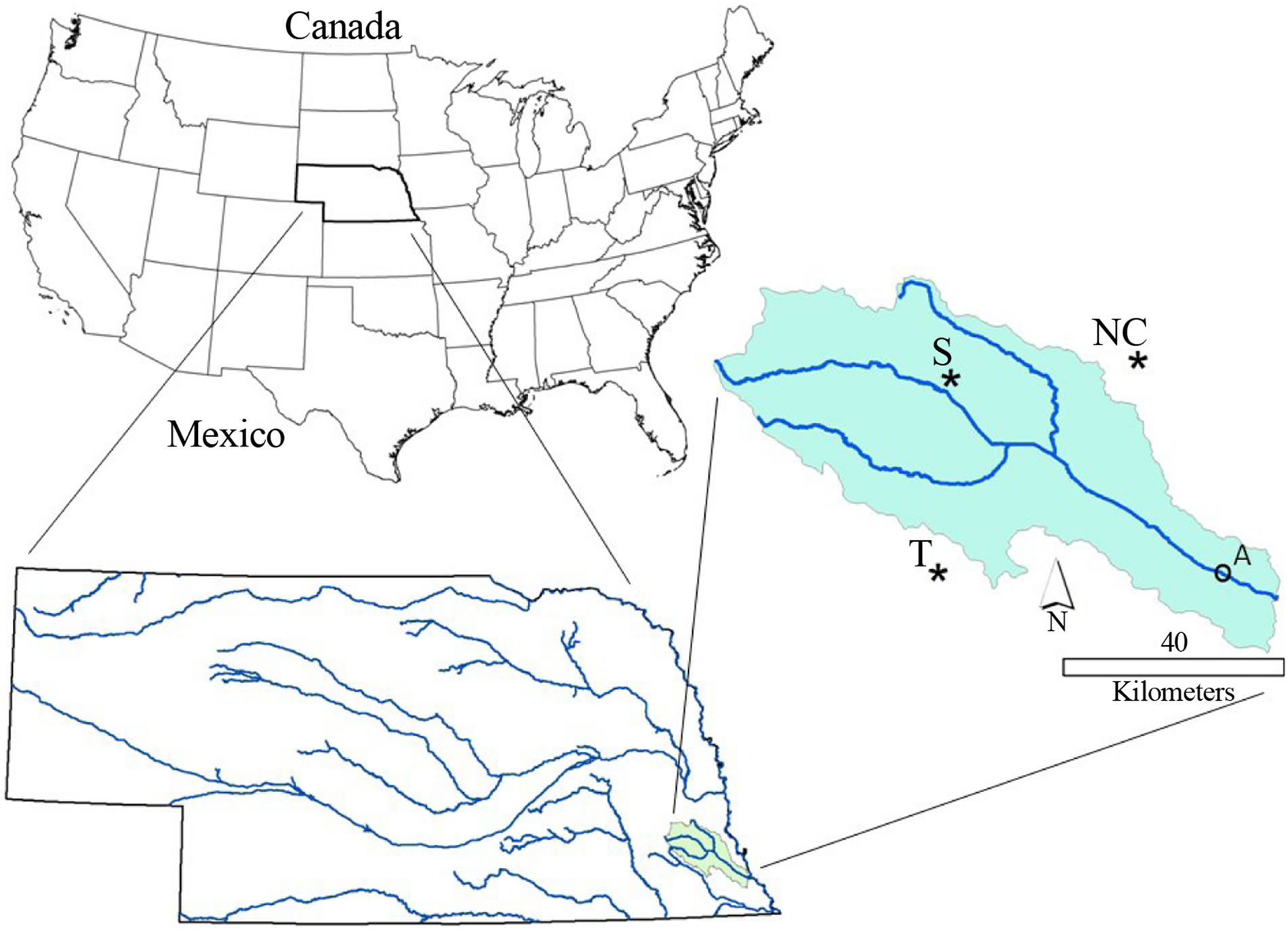
Figure 1. Location of the Little Nemaha watershed within Nebraska, USA. Daily precipitation and temperature are measured at Auburn (A), Nebraska City (NC), Syracuse (S) and Tecumseh (T). Daily streamflow rates are from USGS station at Auburn (A).
air temperature (T) (Figuer 2(a)). Figure 3 displays the spatial distribution of the mean annual P and T values, beside the CREMAP ET rates, at the MODIS grid-resolution, obtained by spatial interpolation, using inverse-distance weighting of the values measured at the four climate stations of Figure 1. The area is part of the dissected plains region of Nebraska, with a gentle topography underlain by glacial till deposits, with a mean depth to the groundwater of about 15 m from the surface. The predominant physical soil texture at the land surface (generalized from STATSGO data of USDA [14]) is clayey loam turning into loam in the stream valleys. As Figure 2(b) demonstrates, inter-annual variability of precipitation is significant, the 2002-2006 period having had experienced a significant drought.
Daily runoff was simulated by a lumped-parameter conceptual model of Jakeman and Hornberger [15]—JH model for further reference—over the 2003-2008 period, having a complete daily precipitation (as well as temperature, snow depth and snow accumulation) record, and where the starting and ending years denote hydrologic years, beginning in November (the driest non-winter month in Nebraska, see Figure 2(a)), the previous year. The model first transforms the daily precipitation rate, ri (mm·d−1), of day i into “excess rainfall” through the definition of an antecedent precipitation index, si (−) as
 (1)
(1)
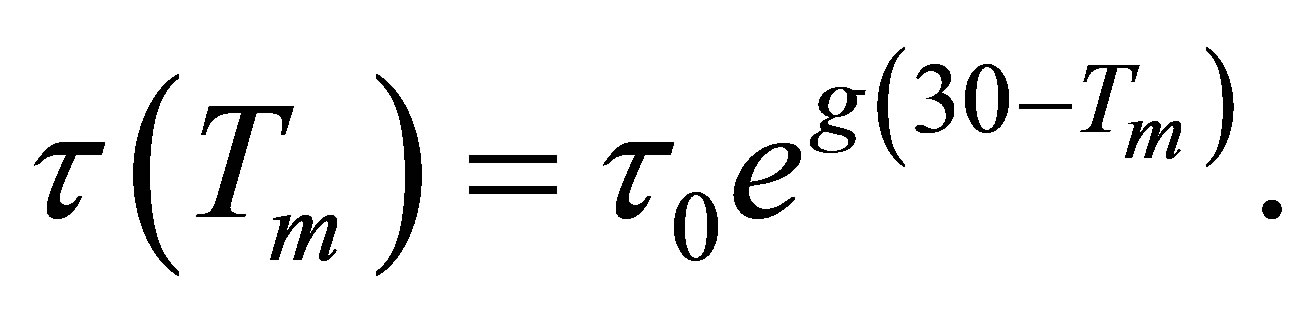
Here c (d mm−1) is just an adjustment factor ensuring that the volume of “excess rainfall” equals the volume of observed runoff over the calibration period. The order of the polynomial in (1) was set to seven through “trial and error”. The variable, τ (−), represents the rate at which
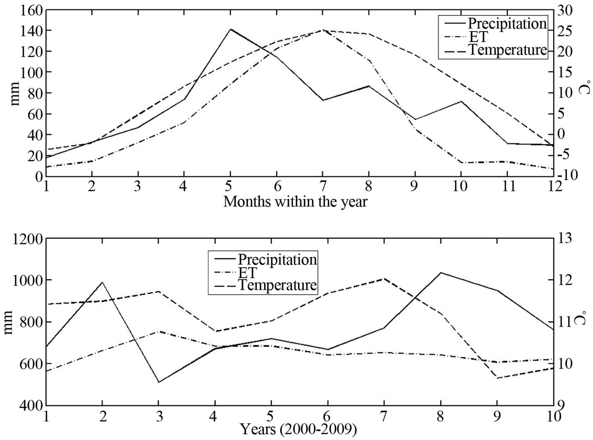
Figure 2. Catchment-averaged values: (a) mean monthly P (mm), CREMAP-derived ET (mm) and T (˚C); (b) annual P (mm), CREMAP-derived ET (mm) and mean T (˚C) of the Little Nemaha watershed for the 2000-2009 period.
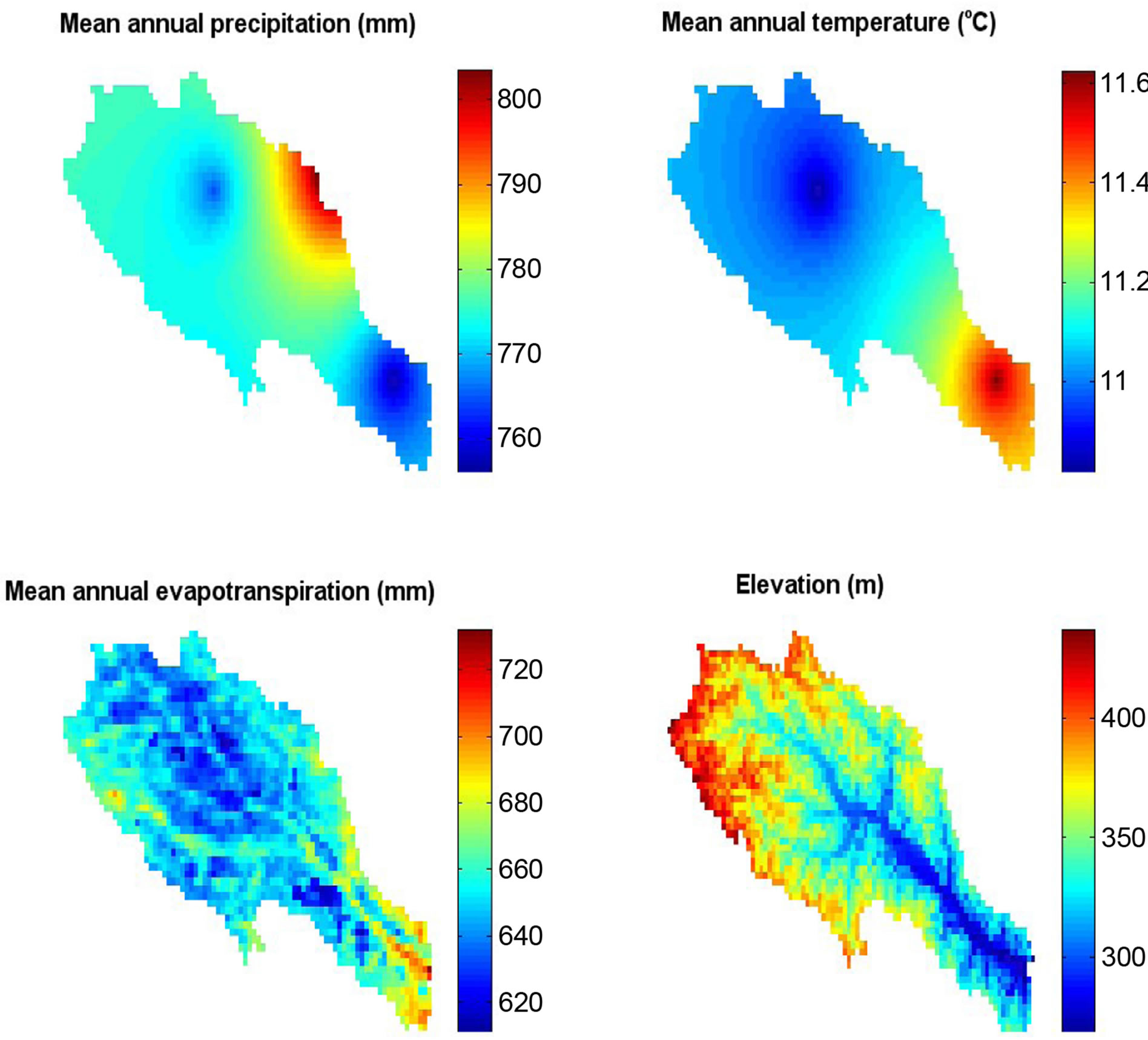
Figure 3. Distribution of the P, T and CREMAP-derived ET (from Szilagyi, et al., 2013a) values over the Little Nemaha catchment for the 2000-2009 period. The elevation (a.m.s.l) distribution at the MODIS resolution is also shown. The catchmentand period-averaged values of P, T and ET are: 775 mm·yr−1, 11˚C, and 650 mm·yr−1, respectively.
catchment wetness declines, a function of the seasons, expressed in the form as
 (2)
(2)
Tm is the catchment-averaged mean air temperature (˚C) in month m (= 1,…,72), g (˚C−1) is a temperature modulation factor, and τ0 is the reference value of τ. Excess rainfall, ui (mm d−1), then obtained as the product of the actual si and ri values, subsequently transformed into runoff via the help of two parallel linear reservoirs, with storage coefficients kq and ks (d−1) for quickand slowflow responses, with simultaneous inputs to them as αui and (1 − α)ui, respectively, where α (−) is a constant multiplier from the (0, 1) range. The original JH model described thus far was amended by considerations of snow. During winter months excess rainfall is taken to be zero on days with reported snow accumulations and is augmented by melt-water of snow, whenever reported snow depth values decrease between consecutive days. By “trial and error” during model calibration (see below) the factor that best transformed reported snow-depth values in mm to water depth in mm was 0.01. This value is a magnitude smaller than the typically applied snow-water equivalent, but it also accounts for any sublimation and evaporation of snow across the watershed before the snow appears as runoff. The resulting model has five parameters to calibrate, i.e., τ0, g, α, kq and ks, similar to the original JH model.
Runoff at the monthly time-scale was simulated by a modified version of a simple distributed-parameter water-balance model of Vorosmarty et al. [16] and Szilagyi and Vorosmarty [17] over the 2000-2009 calendar years. The model tracks the soil moisture, SM (mm), of the root zone of the vegetation with rooting depth, RD (m), and field capacity, FC (−), values specified at each MODIS cell, derived from knowledge of the vegetation type and physical soil texture. Table 1 lists the values employed in this study. Open water surfaces and wetlands did not contribute to runoff, which involved only two cells. The assumed maximum rate of cell ET (ETmax in mm·mo−1) each month was first estimated by the Jansen-Haise [18] equation as
 (3)
(3)
Rs (cal·cm−2·d−1) is the incident solar radiation, n is the number of days within the month, and Tm (˚C) is the monthly mean air temperature of the cell. As an alternative, ETmax was also estimated by the Priestley-Taylor [8] equation as
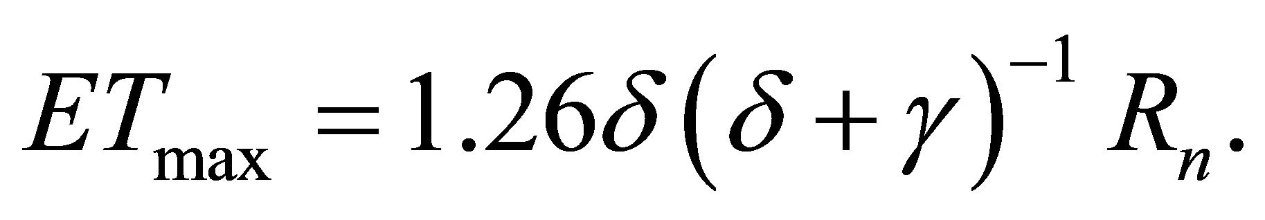 (4)
(4)
δ (hPa·K−1) is the slope of the saturation vapor pressure curve at the monthly mean air temperature, γ (hPa·K−1) is the psychrometric constant and Rn is net radiation (expressed in water-depth equivalent of mm·mo−1) at the surface. The monthly Rn estimates came from the WREVAP model as watershed representative values. The monthly changes in SM (i.e., ΔSM) are calculated as follows
 (5)
(5)
 (6)
(6)
 (7)
(7)
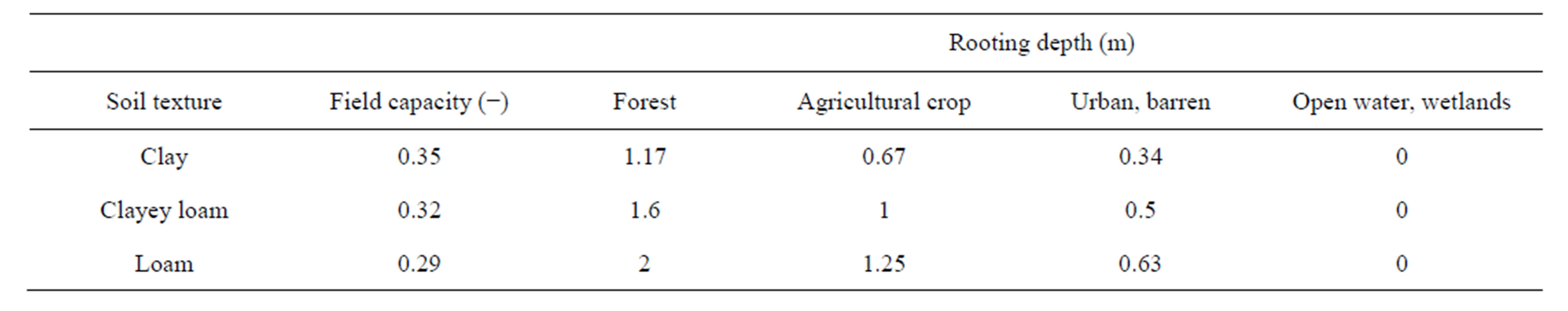
Table 1. Field capacity and rooting depth values employed in the monthly runoff model as functions of physical soil type and/ or vegetation (after Vorosmarty et al. [16]; Szilagyi and Vorosmarty [17]).
β (mm−1), the slope of the moisture-retention curve, empirically estimated as
 (8)
(8)
FC is specified in mm (i.e., FC [mm] = 1000 FC[−]× RD). ET is estimated as ETmax whenever P > ETmax, and as the difference in precipitation rate and (negative) soil moisture change, provided P < ETmax.
Excess monthly rainfall occurs in the model as the difference in estimated SM and FC (mm) in each cell whenever SM > FC (mm), thus reducing SM to FC in such months. The excess rainfall values of the individual cells are subsequently averaged over the cells to obtain one um (m = 1,…, 120) value for each month. A part of excess rainfall [i.e., (1 – α)um] then is routed through a single linear reservoir, representing slow-flow response of the entire catchment (not individual MODIS cells), by expressing α with the help of a power function as
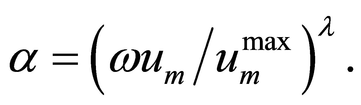 (9)
(9)
 is the largest simulated monthly excess rainfall value, and ω (–) and λ (–) are parameters to be calibrated. Note that quick-flow response, i.e. αum, is not routed in the monthly time-scale. To account for high intensity rains and the ensuing runoff even at the monthly timescale, a constant threshold value, Pth (mm·d−1), was applied above which daily precipitation rates contributed directly (i.e., this portion of the daily precipitation did not go through the soil moisture accounting procedure) to monthly quick-flow response. Note that this way even at the monthly time-step the daily precipitation values were utilized, not typical in modeling at a monthly time-scale. The monthly model has four parameters to calibrate: Pth, ks (mo−1), ω and λ.
Calibration of both models was performed by setting intervals for the individual parameters and trying out different parameter values within those intervals via systematically increasing the parameter values by predefined increments starting at the minimum value of the parameter ranges. The value of the explained variance (R2) in runoff was set as the objective function. As calibration progresses, both the intervals and the increments can successively be decreased once optimal values are reached for each parameter at a given increment value, until a predefined accuracy is reached in the parameter values. Because of the relative shortness of the available data (6 and 10 years, respectively) as well as the low number of flood events, the data periods were not further subdivided into calibration and verification periods, rather, we trained the models with all the available data. Also, the aim was not to use the models for future simulations with the calibrated parameter values but rather to compare their calibrated performances with and without the monthly CREMAP ET data.
The monthly model with the Jensen-Haise equation seriously underestimated runoff by about 60% due to an overestimation of ETmax in general, in comparison with the maximum CREMAP ET values each month. As a result, there could always be found a combination of ω and λ values that improved the R2 and at the same time worsened the ratio of simulated and observed runoff (RR) values ever more slightly, due to a near-flat objective function section in the ω vs λ space. The problem has been avoided by replacing the Jensen-Haise equation with the Priestley-Taylor one. The below results are therefore for this modified version (i.e., employing the Priestley-Taylor equation) of the original model of Vorosmarty et al. [16].
3. Results and Discussion
After calibrating the models (Table 2), both models had to be slightly modified for inclusion of the external ET data and be recalibrated. For the JH model Equation (2) became
 (10)
(10)
ETCR (mm·mo−1) is the watershed-averaged CREMAP ET rate linearly interpolated from the monthly values to the given day;  is the monthly mean air temperature, replaced by zero for months with negative values, and g now is in degree centigrade. By Equation (10) catchment wetness declines fast when it is hot [as with Equation (2)] and humid, i.e., ET is high as well. This last condition is the extra information that comes from the CREMAP ET values. By containing the product of the Tm and ET val-
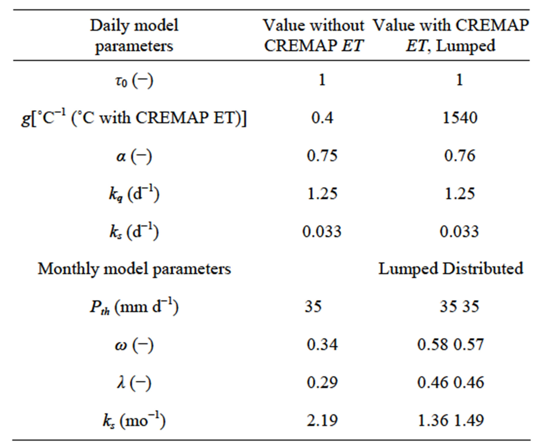
Table 2. Calibrated model-parameter values with and without the inclusion of the lumped or spatially distributed CREMAP ET rates.
ues, and not just the latter, Equation (10) in a way corrects for incorrect ET rates coming from a linear interpolation between consecutive monthly ET values, since in a colder day it can in general be expected that wetness declines in a slower pace (and actual ET is smaller than the interpolated value), and vice versa, on a hot day faster, than what results from the interpolation, derived from average monthly conditions.
In case of the monthly model, ETmax is replaced by the CREMAP cell-ET rate and Equation (7) becomes
 (11)
(11)
utilizing CREMAP ET values, with runoff occurring whenever the updated SM is larger than FC of the given MODIS cell. In the rare occasions when negative SM would occur, the SM value is set to zero. Note that this cannot happen with the analytical solution of Equation (7), describing a linear reservoir with exponentially decaying outflow as SM(t + Δt) = SM(t)exp{β[P(t) − ETmax(t)]}. Table 3 lists the different measures of model performance. For the daily model, inclusion of the watershed-averaged monthly CREMAP ET values left model efficiency practically the same, since the gain is only a few percent at most in any of those measures. This is in accordance with the findings of Oudin et al. [19], who did a similar experiment, since the CREMAP ET values, when averaged over an area (in this case the Little Nemaha watershed) approximate the CR-obtained regional ET rate, the same Oudin et al. [19] applied in their study. The explanation for the current study is that the monthly ET rates cannot fully explain the daily variability of the different physical factors that influence runoff, especially if the physical processes involved are non-linear. Note that the shorter the interval the CR is applied for, the less reliable its predictions, as was noted by Morton et al. [5], which in turn may largely explain why Oudin et al. [19], utilizing the CR at a daily time-step, did not succeed with their runoff simulation improvement experiment. Figure 4 displays the measured and simulated runoff values for a selected period.
At the monthly time-step, however, a slight model improvement is perceptible (Figure 5) with the inclusion of the CREMAP ET rates, either as spatially distributed or catchment-averaged values. Explained variance, R2, increased from 67% to 70%, surpassing the 68% value of the daily model. The root-mean-square-error (RMSE) of the monthly model with lumped or distributed CREMAP
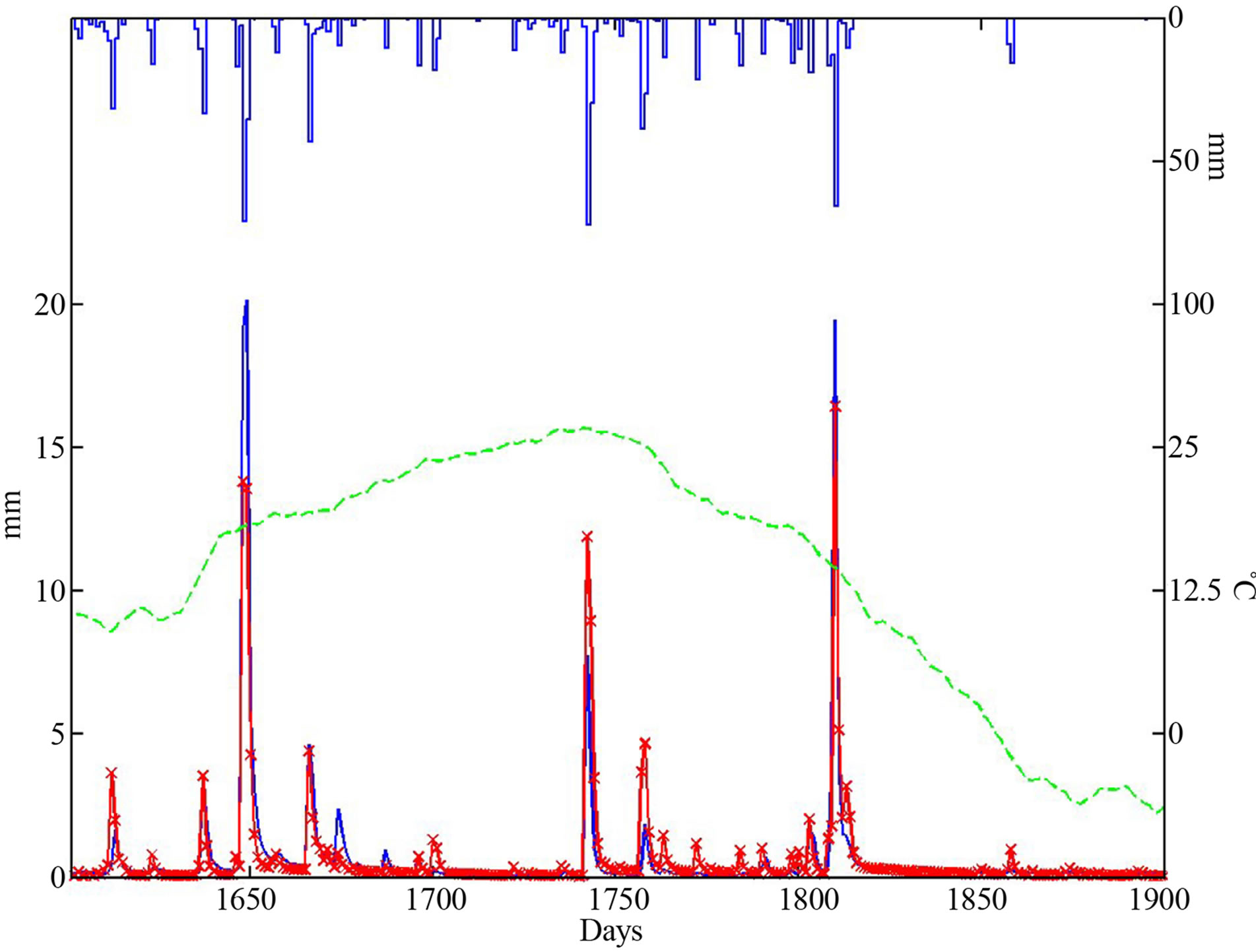
Figure 4. Sample measured (blue line) and simulated (red crosses) daily runoff values (mm) for 20 March 2007-15 January 2008, without the interpolated CREMAP ET rates. Daily precipitation [top blue line (mm)] and air temperature values [green dashes (˚C)] are also shown.
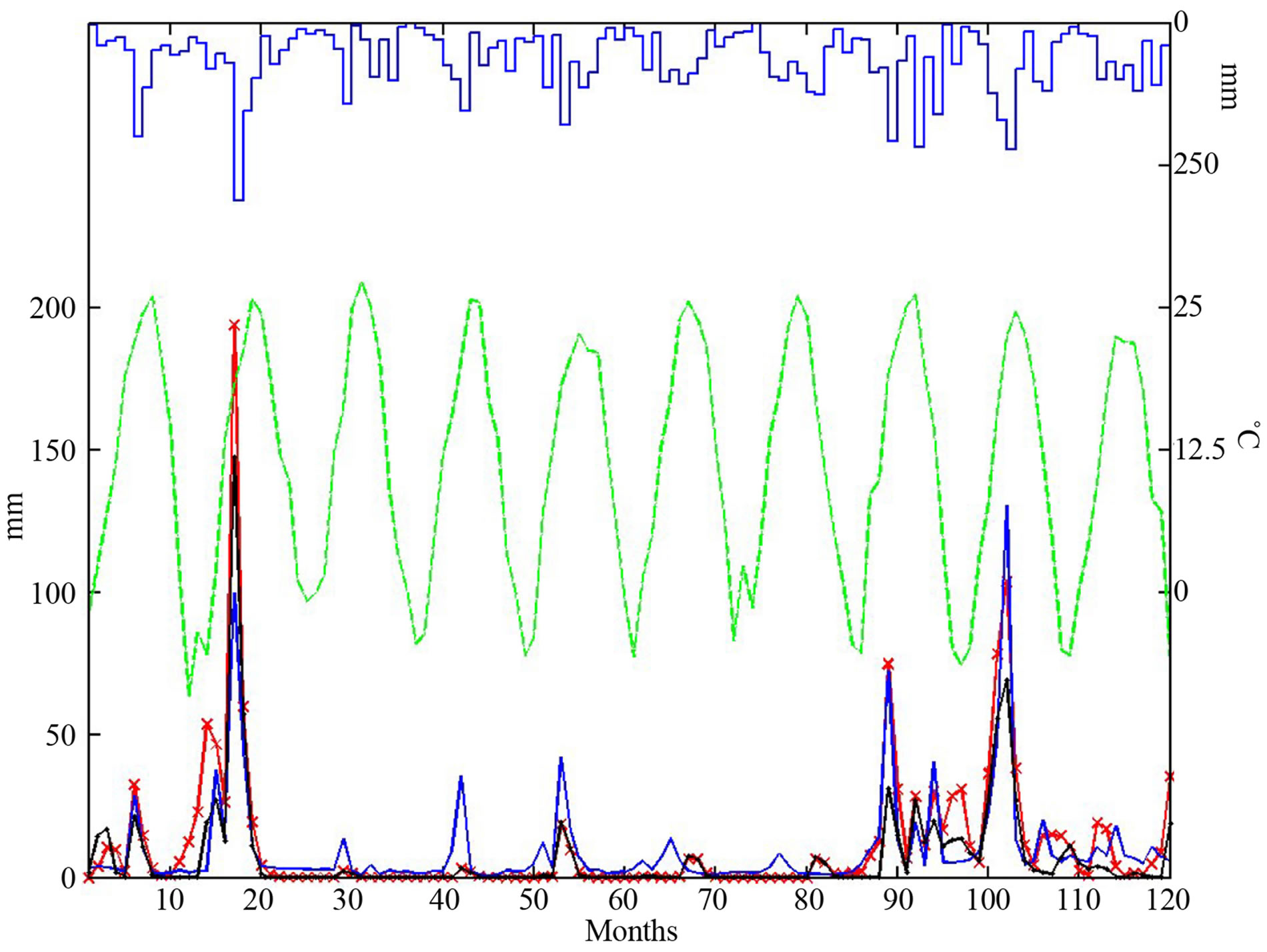
Figure 5. Measured (blue line) and simulated monthly runoff values (mm) from January 2000 to December 2009, with (red crosses) and without (black dots) the spatially distributed CREMAP ET rates. Monthly precipitation [top blue line (mm)] and air temperature values [green dashes (˚C)] are also shown.
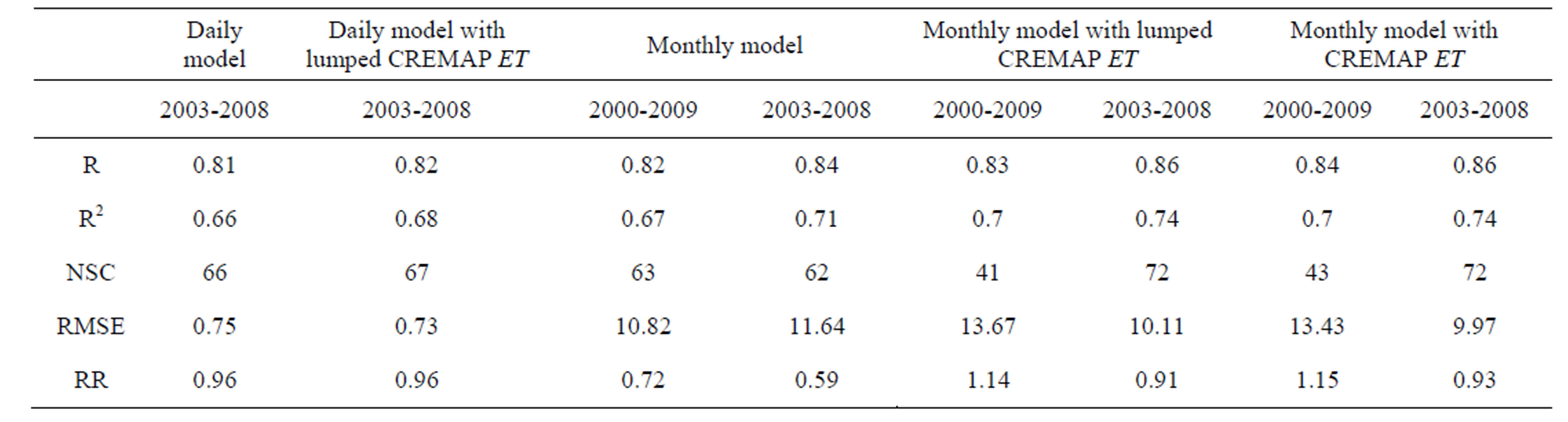
Table 3. Model performance measures: R (−) is correlation coefficient, R2 is explained variance, RMSE (mm) is root-meansquare-error, NSC (%) is the Nash-Sutcliffe performance indicator, RR (−) ratio of modeled and measured runoff over the modeling period (2003-2008 and 2000-2009, respectively).
ET over the 2003-2007 period of the daily model has become smaller (10.11 and 9.97 mm) than that of the daily one (10.27 mm) with its runoff aggregated for the months. A somewhat larger improvement can be seen in the Nash-Sutcliffe model efficiency (NSC = 1 – RMSE2/V, where V is variance of the measured runoff) indicator, i.e., 67% vs 72%, and an even larger one in the R2 values of 0.68 vs 0.74 between the daily and monthly model outputs for the same period. The largest overall change due to the inclusion of CREMAP ET values can be observed in the simulated to measured runoff ratios, both in the 2000-2009 and 2003-2008 periods: from an underestimation of 28% to an overestimation of 14% - 15%, and from an underestimation of 41% to only 7 - 9 percent, respectively. Note that the daily model too has a 4% underestimation even though excess rainfall is tuned via the adjustment factor, c, to the observed runoff volume. A difference in runoff volumes is only possible due to the storage delay of the slow-flow component. The only case when a model performance indicator value listed in Table 3 would not improve with the inclusion of the CREMAP ET values is the NSC value for the entire 2000-2009 period. The sole reason for it is the significant underestimation of watershed ET in month 17 (i.e., May, 2001) with the largest daily and monthly precipitation sums of 79 and 312 mm, respectively, and the largest measured daily runoff rate of ~28 mm, within the period.
It is interesting to note that the lumped monthly CREMAP-ET values yielded practically the same model performance (and similar calibrated parameter values) as the distributed ET rates. The reason must to a certain extent lie in the lumped treatment of the individual cell runoff rates and/or in the fact that different spatial distributions of excess rainfall may indeed generate similar runoff.
Some difference can be found in the calibrated value of the slow-flow storage coefficient between the daily and monthly models. In the daily model average residence time (i.e., ks−1) of water within the ground is about a month, while in the monthly model it is about 15 - 20 days. In the daily model about 25% of the simulated runoff originates from slow-flow response (in either case, with or without CREMAP ET), while in the monthly model it is 44% and 39% (with—either lumped or distributed—or without CREMAP ET). Szilagyi et al. [20], employing an objective base-flow-separation algorithm with long-term (i.e., longer than 30 years) daily discharge measurements at Auburn, Nebraska obtained a base-flow index (i.e., slow-flow contribution to runoff) of about 40% - 45%, close to the current monthly model’s result. Note that in the monthly model, distribution of excess rainfall into quickand slow-flow responses is dependent on the rainfall amounts (Equation (9)), while in the daily model, it is a fixed fraction, set by a constant α value.
4. Conclusion
The focus of the present study was to demonstrate that remote sensing based ET estimates (more specifically the CREMAP ET values of Szilagyi [3]) can be of a quality that may improve existing simple daily rainfall-runoff transformation and/or monthly water-balance model simulation results. While the improvement in the former case was hardly perceptible, it was somewhat more significant in the latter. This is not surprising since the CREMAP ET values are at a monthly time-scale therefore they are not capable of sufficiently recreating the daily variability of ET (as a loss-term) through a simple linear interpolation between consecutive monthly values to estimated daily ET rates, necessary for daily rainfallrunoff transformations. With monthly water-balance calculations this restriction is absent. Future routine application of CREMAP-derived ET rates may boost model efficiency of existing distributed watershed models that run on a monthly basis in areas where the CREMAP method is applicable. The distributed ET rates may also help with the calibration of distributed model parameters, a task not present in the current water-balance model where such parameter values were “a-priori” fixed based on soil and vegetation cover data. The spatially distributed ET estimation method of CREMAP has the distinguished property of not requiring any calibration. The tradeoff is that it cannot be applied over arbitrary areas, e.g., over mountainous and/or arid regions. While remote sensing based ET estimation is a fast evolving arena with ever more complicated and data-intensive methods appearing, typically requiring some sort of calibration based on, e.g. the application of vegetation indices, there is no reason why not to try out and employ existing simple methods, especially if those are calibration-free and therefore add no additional burden to the necessary calibration of the groundwater and/or runoff model in question.
5. Acknowledgements
This work has been supported by the Hungarian Scientific Research Fund (OTKA, #83376) and the Agricultural Research Division of the University of Nebraska. The WREVAP FORTRAN code, with the corresponding documentation, can be downloaded from the personal website of the author (snr.unl.edu/szilagyi/szilagyi.htm).
REFERENCES
- G. B. Senay, S. Leake, P. L. Nagler, G. Artan, J. Dickinson, J. T. Cordova and E. P. Glenn, “Estimating Basin Scale Evapotranspiration (ET) by Water Balance and Remote Sensing Methods,” Hydrological Processes, Vol. 25, No. 26, 2011, pp. 4037-4049. http://dx.doi.org/10.1002/hyp.8379
- J. Szilagyi, A. Kovacs and J. Jozsa, “A Calibration-Free Evapotranspiration Mapping (CREMAP) Technique,” In: L. Labedzki, Ed., Evapotranspiration, INTECH, Rijeka, 2011, pp. 257-274. http://www.intechopen.com/books/evapotranspiration
- J. Szilagyi, “Recent Updates of the Calibration-Free Evapotranspiration Mapping (CREMAP) Method,” In: S. G Alexandris and R. Sticevic, Eds., Evapotranspiration—An Overview, INTECH, Rijeka, 2013, pp. 23-28. http://www.intechopen.com/books/evapotranspiration-an-overview
- R. J. Bouchet, “Evapotranspiration Reelle, Evapotranspiration Potentielle, et Production Agricole,” Annales Agronomae, Vol. 14, 1963, pp. 743-824.
- F. I. Morton, F. Ricard and F. Fogarasi, “Operational Estimates of Areal Evapotranspiration and Lake Evaporation—Program WREVAP,” National Hydrologic Research Institute Paper No. 24, Ottawa, 1985.
- PRISM Climate Group, “Climate Data,” Oregon State Uni- versity, Corvallis, 2004. http://prism.oregonstate.edu
- National Oceanographic and Atmospheric Administration (NOAA), “Surface Radiation Budget Data,” 2009. http://www.atmos.umd.edu/~srb/gcip/cgi-bin/historic.cgi
- C. H. B. Priestley and R. J. Taylor, “On the Assessment of Surface Heat Flux and Evaporation Using Large-Scale Parameters,” Monthly Weather Review, Vol. 100, No. 2, 1972, pp. 81-92. http://dx.doi.org/10.1175/1520-0493(1972)100<0081:OTAOSH>2.3.CO;2
- J. Szilagyi, V. Zlotnik, J. Gates and J. Jozsa, “Mapping Mean Annual Groundwater Recharge in the Nebraska Sand Hills, USA,” Hydrogeology Journal, Vol. 19, No. 8, 2011, pp. 1503-1513. http://dx.doi.org/10.1007/s10040-011-0769-3
- J. Szilagyi, A. Kovacs and J. Jozsa, “Estimation of Spatially Distributed Mean Annual Recharge Rates in the Danube-Tisza Interfluvial Region of Hungary,” Journal of Hydrology and Hydromechanics, Vol. 60, No. 1, 2012, pp. 64-72.
- J. Szilagyi and J. Jozsa, “MODIS-Aided Statewide Net Groundwater-Recharge Estimation in Nebraska,” Ground Water, Vol. 51, No. 5, 2013, pp. 735-744.
- J. Szilagyi, V. Zlotnik and J. Jozsa, “Net Recharge versus Depth to Groundwater Relationship in the Platte River Valley of Nebraska, USA,” Ground Water, Vol. 52, No. 1, 2014, in Press.
- P. Dappen, I. Ratcliffe, C. Robbins and J. Merchant, “Map of 2005 Land Use of Nebraska,” 2007. http://www.calmit.unl.edu/2005landuse/statewide.shtml
- United States Department of Agriculture, “State Soil Geographic (STATSGO) Data Base,” United States Department of Agriculture, Washington DC, 1991.
- A. J. Jakeman and G. M. Hornberger, “How Much Complexity Is Warranted in a Rainfall-Runoff Model,” Water Resources Research, Vol. 29, No. 8, 1993, pp. 2637-2649. http://dx.doi.org/10.1029/93WR00877
- C. Vorosmarty, B. Moore, A. L. Grace and P. Gildea, “Continental-Scale Models of Water Balance and Fluvial Transport: An Application to South America,” Global Biogeochemical Cycles, Vol. 3, No. 3, 1989, pp. 241-265. http://dx.doi.org/10.1029/GB003i003p00241
- J. Szilagyi and C. J. Vorosmarty, “Water-balance Modelling in a Changing Environment: Reductions in Unconfined Aquifer Levels in the Area between the Danube and Tisza Rivers in Hungary,” Journal of Hydrology and Hydromechanics, Vol. 45, No. 5, 1997, pp. 348-364.
- M. Jensen and H. Haise, “Estimating Evapotranspiration from Solar Radiation,” Journal of Irrigation and Drainage Engineering, Vol. 89, No. IR-4, 1963, pp. 15-41.
- L. Oudin, C. Michel, V. Andreassian, F. Anctil and C. Loumagne, “Should Bouchet’s Hypothesis Be Taken into Account in Rainfall-Runoff Modelling? An Assessment over 308 Catchments,” Hydrological Processes, Vol. 19, No. 20, 2005, pp. 4093-4106. http://dx.doi.org/10.1002/hyp.5874
- J. Szilagyi, E. F. Harvey and J. Ayers, “Regional EstimaTion of Base Recharge to Ground Water Using Water Balance and a Base-Flow Index,” Ground Water, Vol. 41, No. 4, 2003, pp. 504-551. http://dx.doi.org/10.1111/j.1745-6584.2003.tb02384.x