Open Journal of Acoustics
Vol.3 No.3(2013), Article ID:36738,5 pages DOI:10.4236/oja.2013.33010
The Corrected Expressions for the Four-Pole Transmission Matrix for a Duct with a Linear Temperature Gradient and an Exponential Temperature Profile
School of Mechanical Engineering, The University of Adelaide, Adelaide, Australia
Email: *carl.howard@adelaide.edu.au
Copyright © 2013 Carl Q. Howard. This is an open access article distributed under the Creative Commons Attribution License, which permits unrestricted use, distribution, and reproduction in any medium, provided the original work is properly cited.
Received May 28, 2013; revised June 28, 2013; accepted July 5, 2013
Keywords: Duct; Transmission Matrix; Four-Pole; Temperature Gradient; Finite Element Analysis
ABSTRACT
The purpose of this letter is to present the corrected expressions for the four-pole transmission matrix for a duct with a linear temperature gradient and an exponential temperature profile, described in Sujith [1]. The corrected equations are used in the analyses of a duct that is driven by a piston at one end and a rigid termination at the other end and the gas has a linear and exponential temperature gradients. The acoustic pressure and particle velocity along the duct are calculated and the theoretical results are compared with predictions using finite element analysis.
1. Introduction
The four-pole, or transmission line method is a useful theoretical tool for the acoustic analysis of duct systems with plane waves [2,3].
Sujith [1] described the four-pole transmission matrix for a duct with a linear temperature gradient and an exponential temperature profile. It was found that several of the equations were incorrect and have been corrected here. Simulations of a duct with a linear and exponential temperature profiles were conducted using the theoretical models implemented in Matlab and finite element analysis using Ansys Mechanical APDL and the results agreed.
2. Duct with a Linear Temperature Profile
Consider a duct filled with a gas that has linear temperature profile given by
 (1)
(1)
where is the gradient of the temperature profile, and
  is the temperature at
 . The speed of sound and density of the gas vary with temperature as [4]
 (2)
(2)
 (3)
(3)
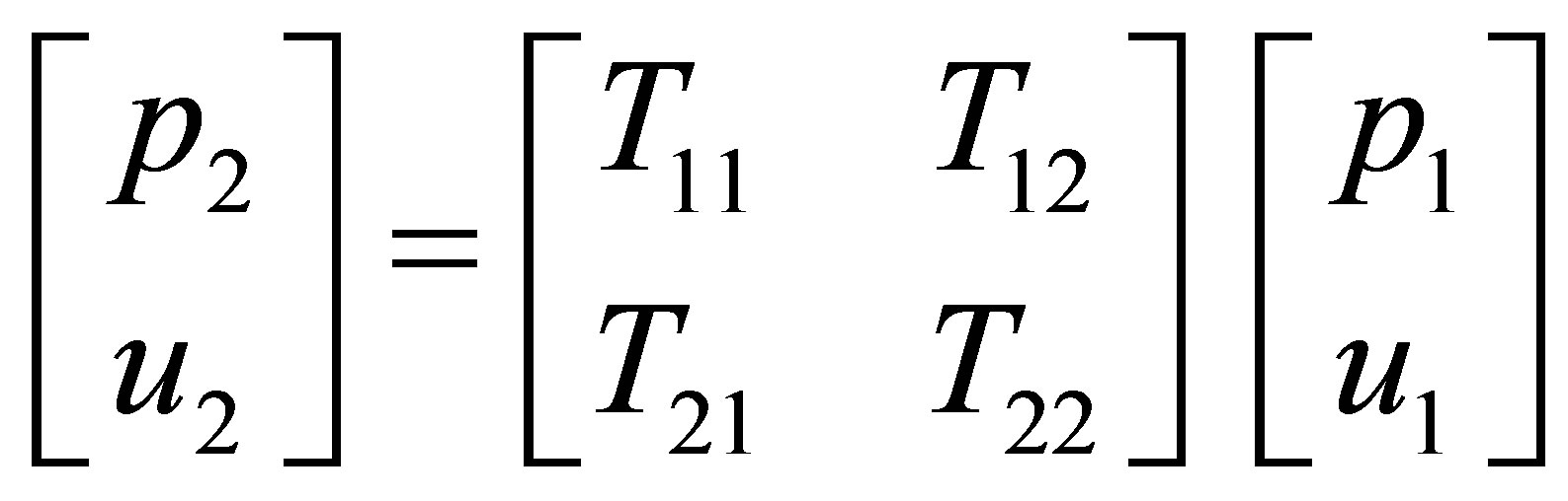
The pressure and acoustic particle velocities at the ends of the duct are related by the four-pole transmission matrix as
 (4)
(4)
Where pi and ui are the acoustic pressure and acoustic particle velocity at the ends of the duct, respectively. The equations presented by Sujith [1] do not include terms for the cross-sectional area of the inlet and outlet of the duct, which is usually included in transmission matrix formulations, such as [5]. By following the derivation presented in Sujith [1], using the software package Mathcad to perform the algebraic manipulations, and using the Wronskian relationship [6]
 (5)
(5)
The elements of the four-pole transmission matrix are
 (6)
(6)
 (7)
(7)
 (8)
(8)
 (9)
(9)
where the specific gas constant is  and the constant
 ![]() is
is
 (10)
(10)
Equations (7) and (8) presented here are the corrected versions of Equations (14) and (15) in Sujith [1].
Note that if one were to define a constant temperature profile in the duct, such that  and
and , the terms
  and
and  in Equations (7) and (8) equate to
 , and Equation (10) equates to zero which causes numerical difficulties. Instead, an approximation to a constant temperature profile can be made by specifying a small temperature difference between the ends of the duct, say 0.1˚C. It can be shown numerically that this will approximate the transmission matrix for a duct with a constant temperature profile and the same cross-sectional areas at the inlet and outlet of the duct given by [5]
 (11)
(11)
3. Duct with an Exponential Temperature Profile
Sujith [1] also describes the four-pole transmission matrix for a duct with an exponential temperature profile given by
 (12)
(12)
The equation for the acoustic pressure along the duct is given by
 (13)
(13)
The equation for the acoustic particle velocity is given by
 (14)
(14)
 (15)
(15)
 (16)
(16)
Equation (15) presented here is the corrected version of Equation (20) in Sujith [1]. Following the same derivation in Sujith [1], using Mathcad to perform the algebraic manipulations, and using Equation (5), the elements of the transmission matrix are
 (17)
(17)
 (18)
(18)
 (19)
(19)
 (20)
(20)
where
 (21)
(21)
 (22)
(22)
 (23)
(23)
Equations (17) to (20) presented here are the corrected versions of Equations (21) to (24) in Sujith [1].
4. Finite Element Analysis
A finite element model of a duct with a piston excitation at one end and rigid termination at the other end was created using the finite element analysis software Ansys, release 14.5. A capability introduced in release 14.5 is the ability to define acoustic elements that have temperatures defined at nodes. In previous releases of the software, the speed of sound and density of the gas had to be defined using a set of material properties. A model of duct with temperature variations could only be created using small duct segments with constant material definitions in each segment. Hence, an impedance discontinuity would have been created at the interface between two duct segments with dissimilar material properties, and would have caused acoustic reflections due to the impedance mismatch at the interface. The new capability enables one to define a temperature gradient across an element so that there is no impedance discontinuity.
The process for conducting an acoustic finite element analysis where there are variations in the temperature of the gas involves several steps as follows:
1) A solid model is created that defines the geometry of the system.
2) The solid model is meshed with thermal elements (SOLID70).
3) The temperature boundary conditions are applied for each region.
4) A static thermal analysis is conducted to calculate the temperature distribution throughout the duct network.
5) The temperatures at each node are stored in an array.
6) The thermal elements are replaced with acoustic elements (FLUID30).
7) The values of temperatures stored in the array are used to define the temperature at each node.
8) Anechoic boundary conditions are set at the duct inlet and outlet (using the MAPDL command SF, IMPD, INF).
9) The acoustic velocity at the duct inlet is defined (using the MAPDL command SF, SHLD, velocity).
10) A harmonic analysis is conducted over the analysis frequency range.
11) The sound pressure levels at the duct inlet, outlet, and the entrance and closed end of the QWT are calculated.
Table 1 lists the parameters of the duct where there was a linear temperature gradient.
Figure 1 shows the finite element mesh of the circular duct created using Ansys Mechanical APDL. Figure 2 shows the results from conducting a static thermal analysis, where the temperatures at the inlet and outlet of the duct were set as boundary conditions that causes a linear temperature profile in the duct. The calculated nodal temperatures from the thermal solid elements are used to de-

Table 1. Parameters used in the analysis of a piston-rigid circular duct with a linear temperature gradient.
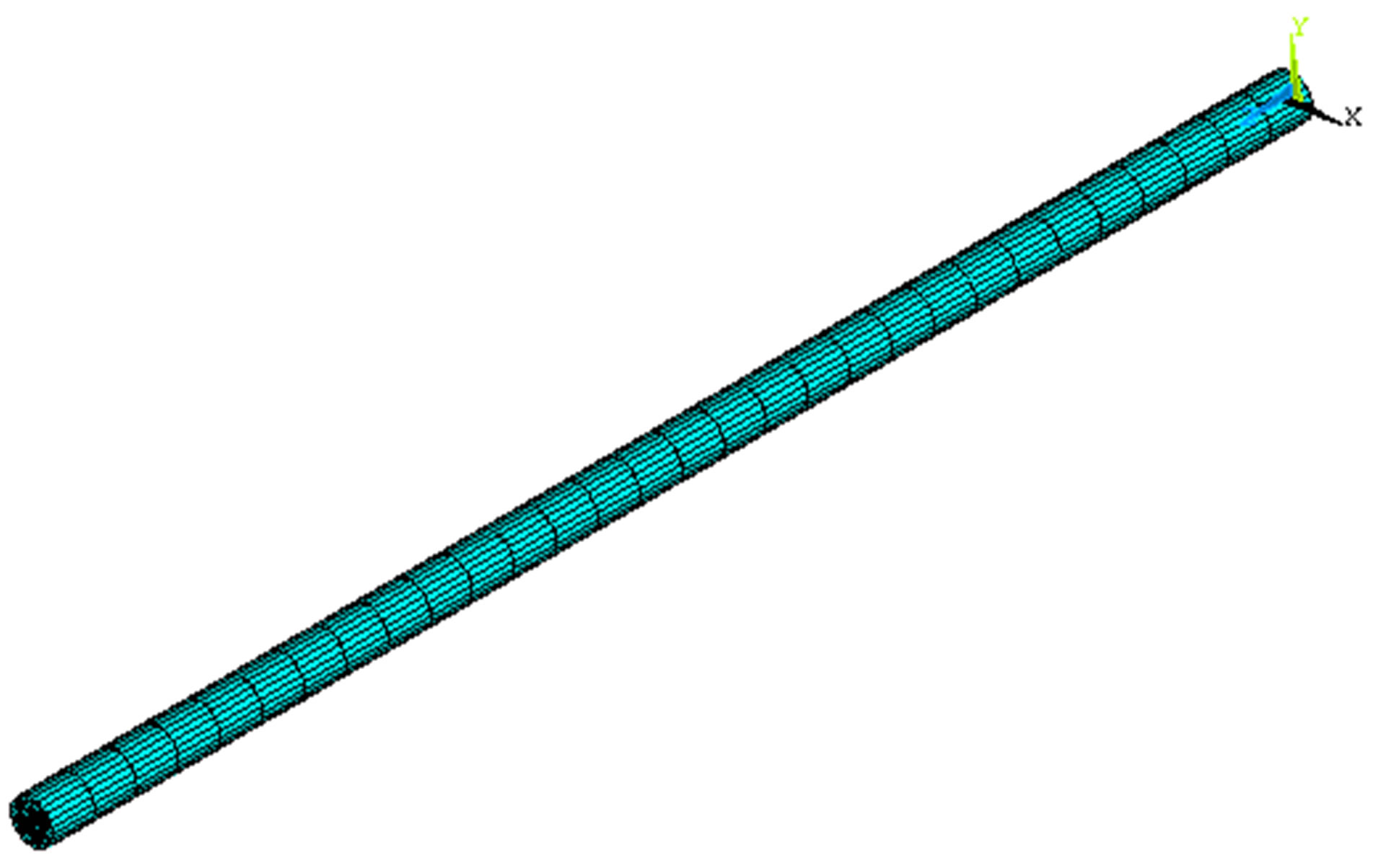
Figure 1. Finite element mesh of the duct.
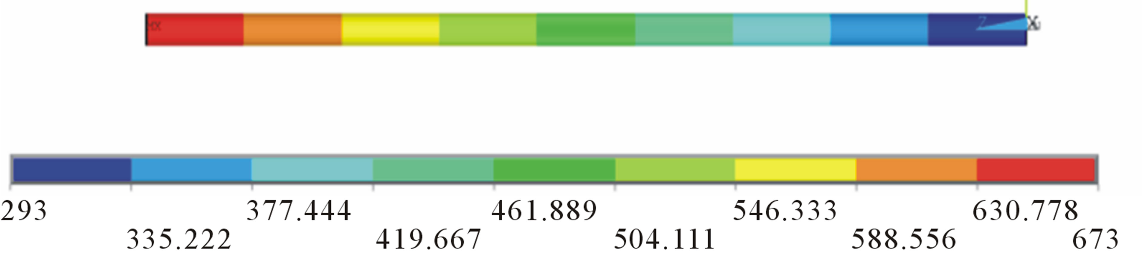
Figure 2. Linear temperature gradient of the gas in the duct where the temperature contours are in Kelvin.
fine the temperature at the nodes of the acoustic elements.
5. Comparison of Theoretical and FEA Predictions
A circular duct with a piston at one end and a rigid termination at the other was modeled theoretically usingMatlab, and using finite element analysis, using Ansys Mechanical APDL release 14.5.
Figure 3 shows the comparison of the sound pressure level in the duct calculated using the theoretical model and Ansys Mechanical APDL for the cases where the temperature of the gas in the duct was:
• at an elevated temperature of 400˚C;
• at an ambient temperature of 22˚C;
• a linear temperature gradient of 400˚C at the rigid end and 20˚C at the piston end.
Figure 4 shows the comparison of the sound pressure level in the duct calculated using theory and Ansys Mechanical APDL when there was an exponential temperature profile of the gas between T1 = 1000˚C = 1273 K at the rigid end and T2 = 20˚C = 293 K at the piston end.
The Ansys Mechanical APDL results agree with the theoretical predictions. Comparisons were also made between theoretical and Ansys predictions of the real and imaginary parts of the acoustic pressure and acoustic particle velocity and all the results agreed.

Figure 3. Sound pressure level in a piston-rigid duct at 22˚C, 400˚C, and linear temperature gradient 400˚C to 20˚C.
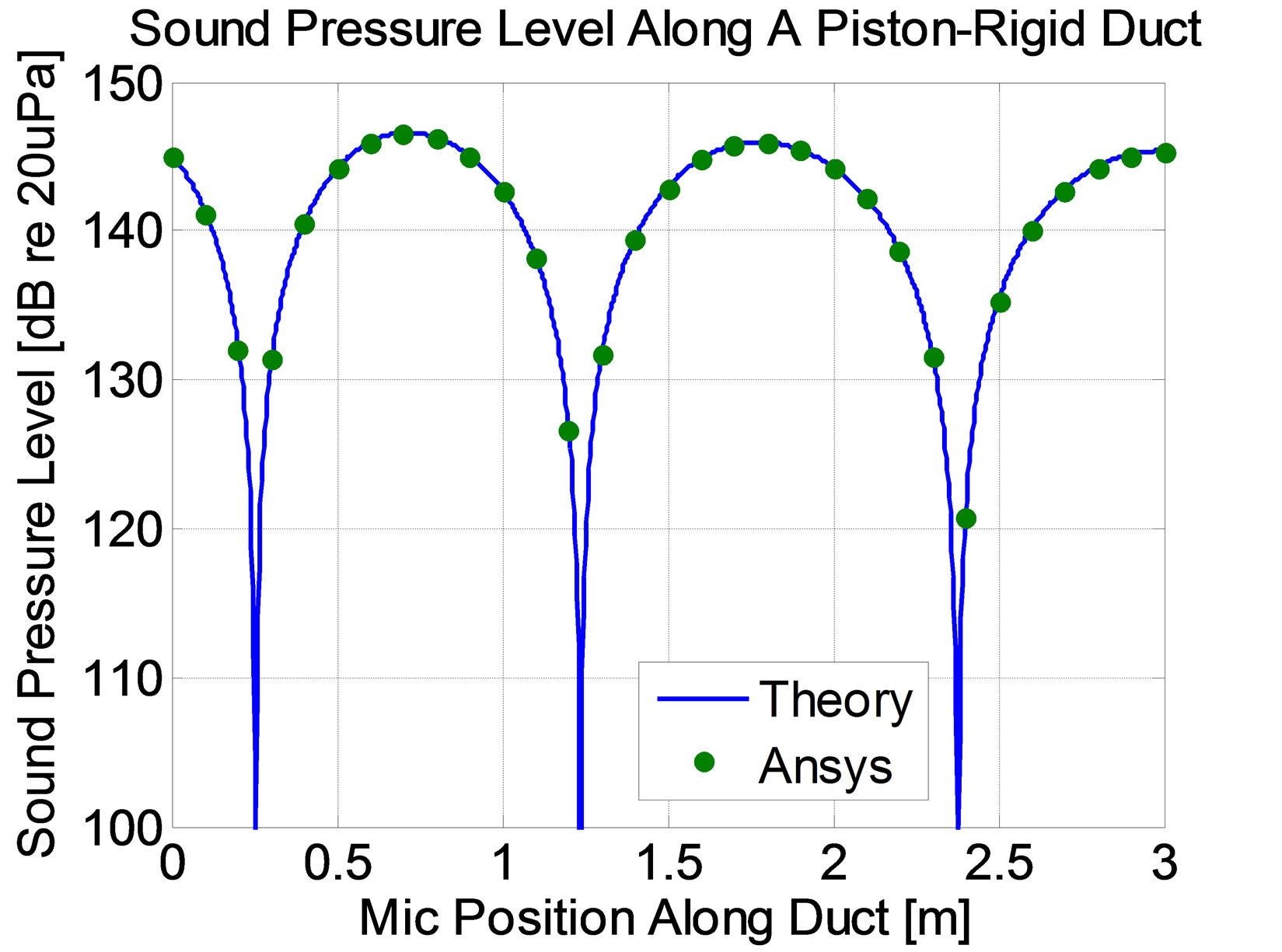
Figure 4. Sound pressure level in a piston-rigid duct when there was an exponential temperature profile from 1000˚C to 20˚C.
6. Conclusion
The corrected equations are presented from Sujith [1] for the four-pole transmission matrix for the cases of a linear temperature gradient and an exponential temperature profile. The predictions using the theoretical models for the cases of a linear and exponential temperature profiles in a duct with a piston at one end and rigid termination at the other agreed with results from finite element analyses.
REFERENCES
- R. I. Sujith, “Transfer Matrix of a Uniform Duct with an Axial Mean Temperature Gradient,” The Journal of the Acoustical Society of America, Vol. 100, No. 4, 1996, pp. 2540-2542. doi:10.1121/1.417362.
- M. L. Munjal, “Acoustics of Ducts and Mufflers with Application to Exhaust and Ventilation System Design,” Section 2.18, Wiley-Interscience, New York, 1987.
- A. G. Galaitsis and I. L. Ver, “Chapter 10: Passive Silencers and Lined Ducts,” In: L. L. Beranek and I. L. Ver, Eds., Noise and Vibration Control Engineering: Principles and Application, Wiley Interscience, New York, 1992, pp. 367-427.
- D. A. Bies and C. H. Hansen, “Engineering Noise Control: Theory and Practice,” 4th Edition, Spon Press, London, 2009. pp. 17-18, Equations (1.8).
- A. G. Galaitsis and I. L. Ver, “Chapter 10: Passive Silencers and Lined Ducts,” In: L. L. Beranek and I. L. Ver, Eds., Noise and Vibration Control Engineering: Principles and Application, Wiley Interscience, New York, 1992, p. 377, Equations (10.15).
- F. W. J. Olver, “Handbook of Mathematical Functions with Formulas, Graphs, and Mathematical Tables,” Dover Publications, New York, 1972, p. 360, Equation (9.1.16).
List of Symbols
a: radius of the duct b: constant in Equation (12)
c0: speed of sound at ambient temperature
 : speed of sound at each end of the duct
 : constants in Equations (22) and (23)
 : unit imaginary number
 : Bessel function of the nth order
 : wave-number
![]() : length of the duct
: length of the duct
 : molecular weight of air
 : pressure at the ends of the duct
 : static pressure in the duct
 : universal gas constant
 : specific gas constant
![]() : cross sectional area of the duct
: cross sectional area of the duct
![]() : temperature of the fluid
: temperature of the fluid
 : temperatures of fluid at the ends of the duct
 : particle velocities at the ends of the duct
 : mass volume velocity at the ends of the duct
 : Neumann function of the n-th order
 : axial coordinate along the duct
![]() : constant in Equation (12)
: constant in Equation (12)
 : density of fluid at ends of duct
ω: angular frequency
ν: constant defined in Equation (10)
 : ratio of specific heats (CP/CV)
NOTES
*Corresponding author.