ABSTRACT

This theoretical paper analytically predicts the existence of new surface wave in propagation direction [101] in the cubic piezoelectromagnetics. The solution for the velocity of the new wave is given in an explicit form. Such new wave possesses one real component and two purely imaginary components. This corresponds to a leaky acoustic SH-wave. However, in this case the real component does not participate in the complete displacements. As a result, the new wave can represent the new shear-horizontal surface acoustic wave (SH-SAW) for suitable boundary conditions. For the mechanically free surface, several combinations of the following electrical and magnetic boundary conditions were used: Electrically closed, electrically open, magnetically closed, magnetically open surface. This new SH-SAW can propagate with the speed slightly larger than that for the SH bulk acoustic wave coupled with both the electrical and magnetic potentials. The existence conditions for the new SH-SAW were also discussed. They can be very complicated and depend on all the material parameters. It was also discussed that the results can be true for the left-handed metamaterials. It is thought that the new SH-SAW can be produced by electromagnetic acoustic transducers (EMATs) because generation of SH-SAWs is feasible with the EMATs. This can be a problem for experimentalists working in the research arenas such as acoustooptics, photonics, and acoustooptoelectronics.

1. Introduction

There is a continuous interest in the various theoretical and experimental investigations of the magnetoelectric (ME) effect in (composite) materials for development of smart materials in the microwave technology. To start a short historical review of works on the magnetoelectric effect, it is possible first of all to mention several classical works [1-5] published in 1970s which have originally studied composite materials and the ME effect. Indeed, piezoelectrics and piezomagnetics can be bonded together in different ways to form composites that exhibit the ME effect. The ME effect can lead to the following: An electrical signal caused by the presence of the piezoelectric phase of such composites can be obtained as a result of the application of a magnetic field affecting the composite piezomagnetic phase. On the other hand, the composite piezomagnetic phase can magnetically respond because of the application of an electrical field to the ME composite possessing the piezoelectric phase.

It is thought that it is unnecessary to review all the theoretical and experimental works concerning the ME effect and creation and characterization of new two-phase ME composites. One can readily find thousands of papers on the subject. Therefore, it is suitable to give only several review papers on the subject. Indeed, the reader can find that the recent reviews cited in Refs. [6-11] contain enough citations. For the reader who would like to know more about the subject, it is strongly recommended to use the following several additional review papers cited in Refs. [12-15]. According to review paper [9] by Fiebig, such two-phase ME composites are potential candidates for utilization as various acoustic devices, magnetic-field probes, and hydrophones, in electronic packaging and medical ultrasonic imaging, also as sensors and actuators. However, all these review papers did not mention achievements in the theory of the wave propagation in the piezoelectromagnetic composite materials possessing the ME effect.

Concerning the theoretical investigations of the propagation problems of shear-horizontal surface acoustic waves (SH-SAWs), it is essential to mention the excellent work [16] published in 2007 by Arman Melkumyan. In his theoretical work, he discovered twelve new SHSAWs propagating on the free surface of the transversely isotropic piezoelectromagnetics. Treating the wave propagation in these piezoelectromagnetics, Ref. [17] has also introduced seven new SH-SAWs and also confirmed that the SH-SAW called the surface Bleustein-Gulyaev-Melkumyan (BGM) wave can propagate in such piezoelectromagnetics. It is worth noticing that the surface BGMwave in piezoelectromagnetics is analogous to the wellknown surface Bleustein-Gulyaev (BG) wave [18,19] propagating in the transversely isotropic piezoelectrics. Moreover, recent book [20] has analytically found that the BGM-wave can also propagate in the cubic piezoelectromagnetics. This book published in 2011 has also discovered seven new SH-SAWs propagating on the surface of the cubic piezoelectromagnetics and discussed the main differences between the wave propagations in the cubic piezoelectromagnetics and the transversely isotropic piezoelectric composite materials. Note that the wave propagations in cubic piezomagnetics [21] and cubic piezoelectrics [22] are also different from those in the transversely isotropic materials. Also, Ref. [23] has stated that SH-SAWs can easily be produced by electromagnetic acoustic transducers (EMATs). According to books [24, 25], the EMATs offer a series of advantages over traditional piezoelectric transducers. So, the EMATs can be used for measurements of SH-SAW characteristics when the wave propagations in the piezoelectrics, piezomagnetics, or piezoelectromagnetics are studied.

It is thought that there is a lack of works on existence of leaky acoustic waves propagating in piezoelectromagnetics. The leaky acoustic waves, also called the leaky surface acoustic waves (LSAWs), are also very important in acoustics of solids. Generally, some LSAWs are numerically studied in appropriate piezoelectrics and they are longitudinal, for example, see Refs. [26-31]. The works on the LSAW studies frequently use promising noncubic and nontransversely-isotropic piezoelectric monocrystals such as Quartz, Langasite, LiTaO₃, etc. The longitudinal LSAWs propagating on suitable cuts of piezoelectric monocrystals are at least three-partial. It is well-known that the SH-SAWs such as the surface BGwave are two partial and can propagate only on suitable cuts of piezoelectrics or piezomagnetics. It was also mentioned in Ref. [27] that the LSAWs can be used as one of two possible ways to resolve the problem of movement of mobile communication equipments towards higher frequency range. Indeed, the LSAW speed should be higher than the SAW one, using the same crystal cut and propagation direction.

However, an existence of any SH-LSAW in addition to the SH-SAW was not demonstrated, probably, due to the fact that they are two-partial in pure piezoelectrics. As soon as the wave propagation in piezoelectromagnetics is treated, the SH-waves can become three-partial. So, it is expected that some LSAW propagation can be found in piezoelectromagnetics. The main purpose of this report is to analytically demonstrate a possible existence of new SH-wave propagating in the cubic piezoelectromagnetics on the same cuts in addition to the seven new SH-SAWs discovered in the recent book cited in Ref. [20]. It is also noted that the experimental investigations of cubic piezoelectromagnetics are performed not frequently compared with those of the transversely isotropic materials. Therefore, phase velocity calculations for the new SH-wave propagating in concrete cubic piezoelectromagnetics will be not carried out in this report. Note that one can find a proposal of several new cubic piezoelectromagnetic composite materials in book [20]. The following section provides the theoretical description of the problem.

2. Theory

Following the theoretical description of SH-SAW propagation in the cubic piezoelectromagnetics described in book [20], it is possible to briefly introduce the problem focusing on the SH-wave. First of all, it is necessary to state that in this case, the piezoelectromagnetic acoustic waves are managed along direction [101] like that in the cubic piezoelectrics [22]. The theory uses the usual quasistatic approximations, the equations of motion, electrostatics and magnetostatics like those described in books [17,20]. The coordinate beginning is positioned at the interface between the cubic piezoelectromagnetics and a vacuum. The rectangular coordinate x₁- and x₂-axes lie in the interface plane and the x₃-axis is directed perpendicular to both the axes. The SH-wave propagate along the x₁-axis and are polarized along the x₂-axis. In the case of the SH-SAW, the waves must damp towards the depth of the composite material, namely along the negative values of the x₃-axis. However, this is not obligatory in the case of the SH-LSAW because at least one partial component of three must have non-SAW behavior. Indeed, the plane wave approximation is used in the theory of SAW and LSAW propagation.

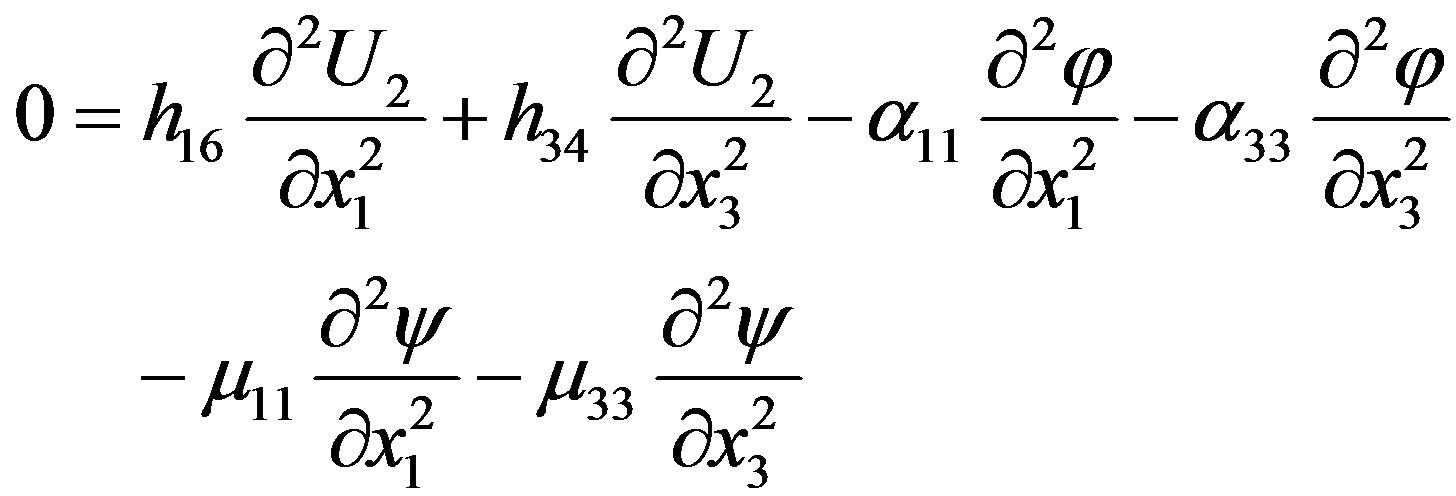
Using only nonzero material constants, it is possible to write the coupled equations of motion for the studied case. They read

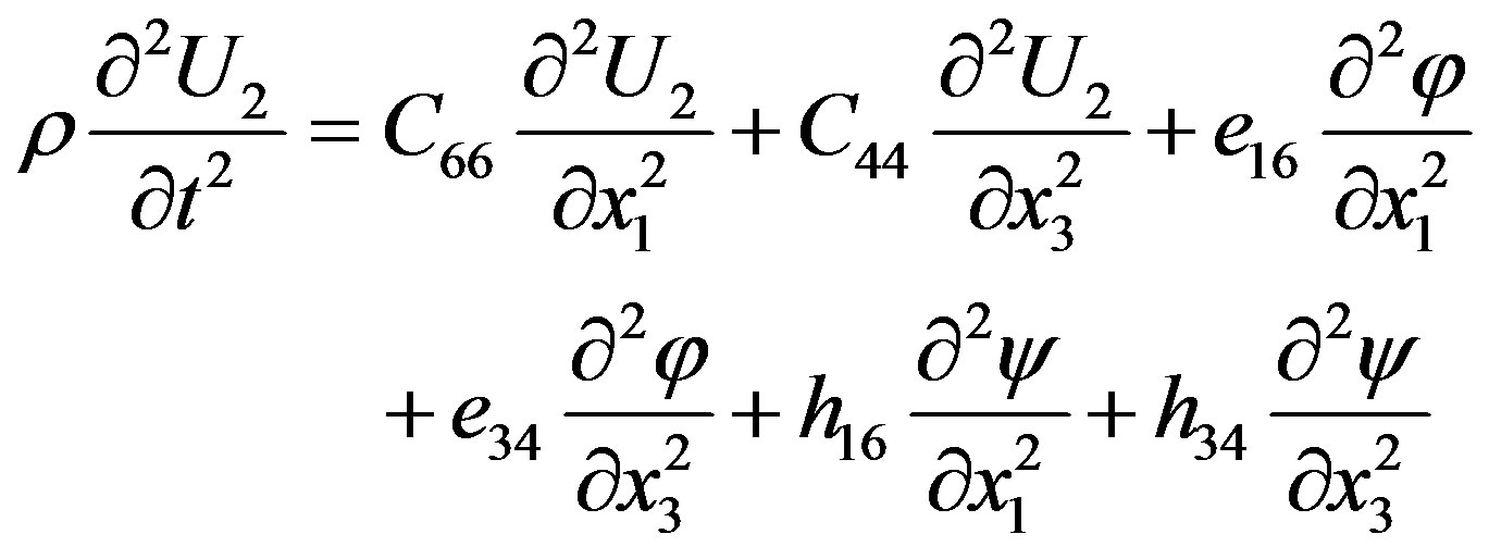(1)

(2)

(3)

In the first equation written above, t stands for time and U₂ is the corresponding component of the mechanical displacement directed along the x₂-axis. Also, φ and ψ are the electrical and magnetic potentials, respectively, defined by E = –¶φ/¶x₃ and H = –¶ψ/¶x₃ where E and H are the electrical and magnetic fields. In the equations written above, the non-zero material constants are as follows: C₄₄ = C₆₆ = C (elastic stiffness constants), e₁₆ = –e₃₄ = e (piezoelectric constants), h₁₆ = –h₃₄ = h (piezomagnetic coefficients), ε₁₁ = ε₃₃ = ε (dielectric permittivity coefficients), μ₁₁ = μ₃₃ = μ (magnetic permeability coefficients), α₁₁ = α₃₃ = α (electromagnetic constants), and r is the mass density.

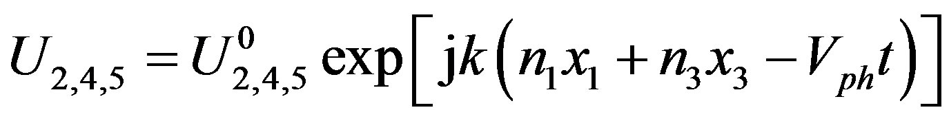
The plane wave solution for the mechanical displacement U₂, electrical potential φ, and magnetic potential ψ can be written in the following form:

(4)

In equation (4), the displacements are defined by U₂ = U, U₄ = φ, U₅ = ψ, and are the initial amplitudes. Also, the directional cosines are n₁ = 1, n₂ = 0, and n₃ ≡ n₃. V_ph and j stand for the phase velocity and the imaginary unity, respectively. The wavenumber k in Equation (4) is coupled with the components {k₁, k₂, k₃} of the wavevector k as follows: {k₁, k₂, k₃} = k {n₁, n₂, n₃}.

Exploiting the solutions in Equation (4) for equations from (1) to (3), the coupled equations of motion can be written in a tensor form. Using the corresponding components of the symmetric GL-tensor in the well-known modified Green-Christoffel equation [32] for brevity, three homogeneous equations can be represented in the following matrix form:

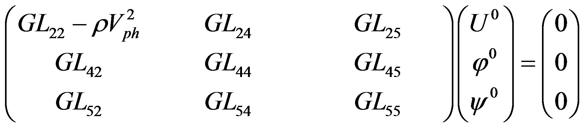(5)

where U⁰ = U₂⁰, φ⁰ = U₄⁰, and ψ⁰ = U₅⁰ represent three components of the eigenvector. Note that the readers themselves can obtain the explicit forms for the GL-tensor components in Equation (5) using plane wave solutions (4) for equations from (1) to (3).

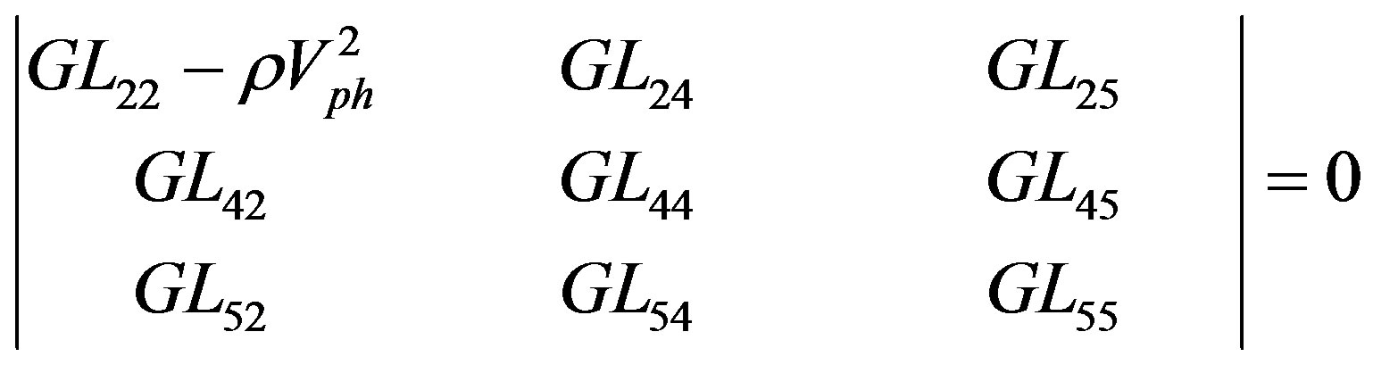
It is obvious that the three-component eigenvector should be nonzero for each eigenvalue n₃ = k₃/k. Suitable eigenvalues n₃ can be obtained when the following matrix determinant of the system of homogeneous Equations (5) becomes equal to zero:

(6)

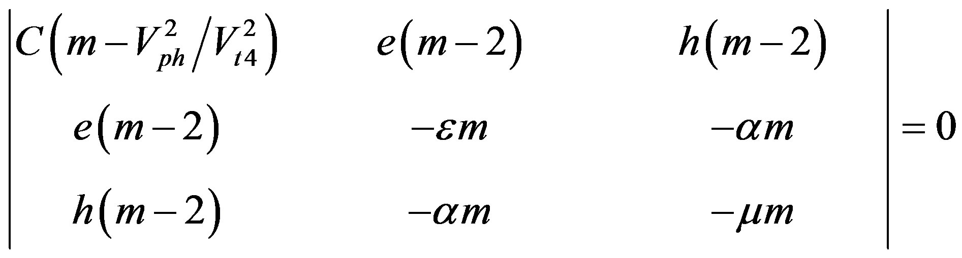
It is useful to rewrite the characteristic determinant in Equation (6) in the following form:

(7)

where m = 1 + sqr(n₃) and V_t4 = sqrt(C/r) is the speed of the bulk acoustic wave (BAW) uncoupled with both the electrical and magnetic potentials.

Analyzing the first row or the first column of the matrix determinant in Equation (7), it is natural to treat the following formula for the new wave velocity:

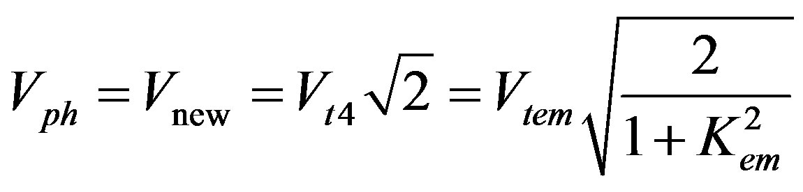(8)

where V_tem = V_t4 sqrt(1 + K_em²) is the speed of the SH-BAW coupled with both the electrical and magnetic potentials because K_em² represents the coefficient of the magnetoelectromechanical coupling (CMEMC). It reads

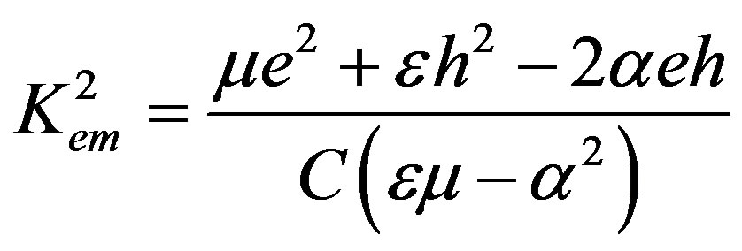(9)

Therefore, the left-hand side in Equation (7) can be written in the form of two factors. The transformed equation can be written as follows:

(10)

The first factor in Equation (10) reveals the following eigenvalue n₃:

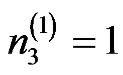(11)

In the studied case of the wave propagation problem, the first eigenvalue in expression (11) can be real. Using it for Equation (5), one can obtain the corresponding eigenvector components. It is apparent that the simplest and most convenient eigenvector components for the first eigenvalue n₃⁽¹⁾ in Equation (11) are

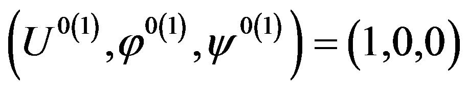(12)

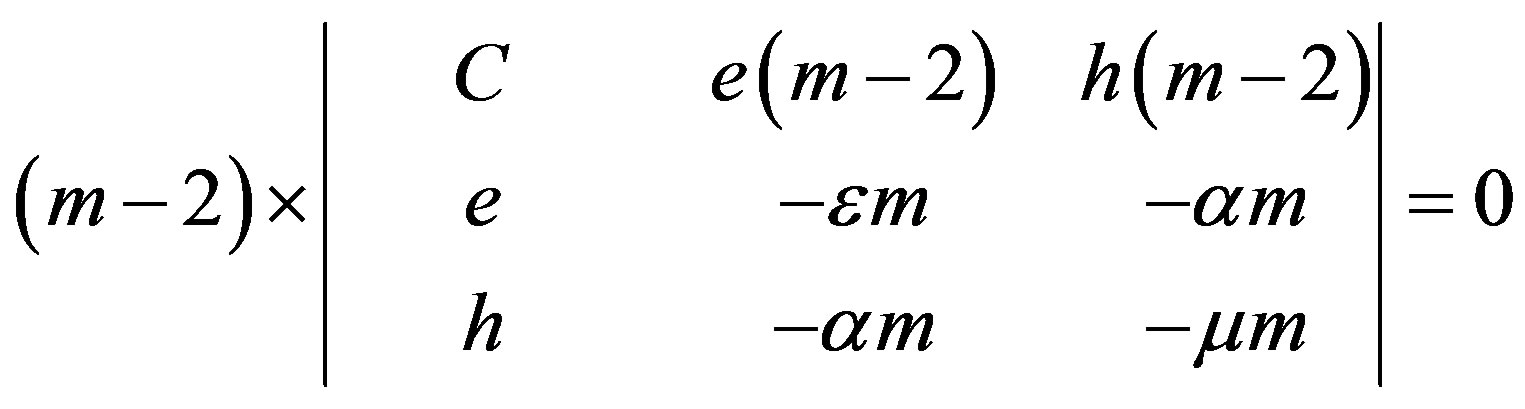
The second factor representing the determinant in Equation (10) can reveal the rest two eigenvalues. Expanding this determinant, one can get the following secular equation:

(13)

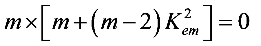
It is clear that Equation (13) also has two factors on the left-hand side. Therefore, the equality in Equation (13) is true when either the first or second factor equals to zero. In the first case of m = 0, the following eigenvalue can be obtained:

(14)

Note that in the wave propagation problem, the sign for the eigenvalue in relation (14) is chosen negative in order to cope with wave motions which must damp towards the depth of the bulk piezoelectromagnetics. This is like the SH-SAW propagation problem. Using the eigenvalue n₃⁽²⁾, one can check that Equation (5) equals to zero with the following eigenvector components:

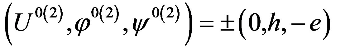(15)

The equality to zero of the second factor in Equation (13) is possible as soon as the eigenvalue n₃ becomes the following function of the CMEMC:

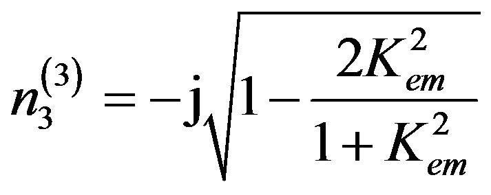(16)

It is crucial to state that it is clearly seen in Equation (16) that for K_em² = 1 one gets n₃⁽³⁾ = 0. This solidly demonstrates that K_em² = 1 results in V_new = V_tem, see expression (8). Therefore, this case is unique and demonstrates some association with the SH-BAW solution. Also, it is apparent that the value of n₃⁽³⁾ becomes real as soon as K_em² > 1 in expression (16). Therefore, it is necessary to cope with K_em² < 1 for simplicity. The case of K_em² = 0 gives n₃⁽³⁾ = n₃⁽²⁾ = –j. This is the case of two equal eigenvectors. This situation always leads to zero value of the boundary-condition determinant and results in zero values of complete displacements. This is like the situation occurred in the cubic piezoelectrics [22], cubic piezomagnetics [21], and cubic piezoelectromagnetics below the SH-BAW velocity V_tem [20]. Therefore, it is possible to state that K_em² = 0 is a unique case, but it is not possible to solidly say that this situation corresponds to an SH-SAW solution.

Utilizing the third eigenvalue defined by relation (16) for Equation (5), one can find that two possible sets of the eigenvector components can exist in this case. The first set of the eigenvector components is expressed as follows:

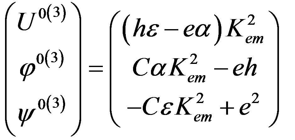(17)

Also, the second set of the eigenvector components can be written as follows:

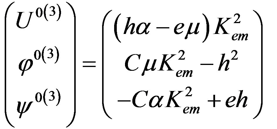(18)

The first problem of the finding of the new SH-wave velocity, eigenvalues, and corresponding eigenvectors was resolved above. The speed of the new SH-wave is given by expression (8). Three eigenvalues n₃ were found in the explicit forms. For the new SH-wave propagation in the cubic piezoelectromagnetics, the first eigenvalue is real and defined by expression (11), but the second and third eigenvalues are purely imaginary and defined by expressions (14) and (16), respectively. Indeed, all the eigenvalues possess the corresponding eigenvectors and the third eigenvalue has two different sets of the eigenvector components.

The second problem is the determination of the existence conditions of the new SH-wave propagation. For this purpose, it is necessary to consider the mechanical, electrical, and magnetic boundary conditions. Al’shits, Darinskii, and Lothe [33] have theoretically studied the two-phase materials and discussed possible boundary conditions for the problem of wave propagation in piezoelectromagnetics. In this case of the wave propagation, it is also possible to use the mechanical boundary condition such as the normal component of the stress tensor at the solid-vacuum interface x₃ = 0 must vanish, following books [17,20]. The electrical and magnetic boundary conditions such as the electrically closed surface (φ = 0) and the magnetically open surface (ψ = 0) can be also applied. These boundary conditions are those which reveal the surface BGM-wave speed in the transversely isotropic piezoelectromagnetic materials [16,17] and the cubic piezoelectromagnetics [20]. The other possible electrical and magnetic boundary conditions are as follows: electrically open surface (D = 0) and the magnetically closed surface (B = 0) where D and B are the normal components of the electrical and magnetic displacements. The mechanical boundary condition used in all the theoretical treatments below is applied to the normal component of the stress tensor, namely σ₃₂(x₃ = 0) = 0 at the interface x₃ = 0 [20] between the crystal surface and a vacuum. This is the case called the mechanically free surface. It is possible to consider possible boundary conditions.

2.1. σ₃₂ = 0, φ = 0, and ψ = 0

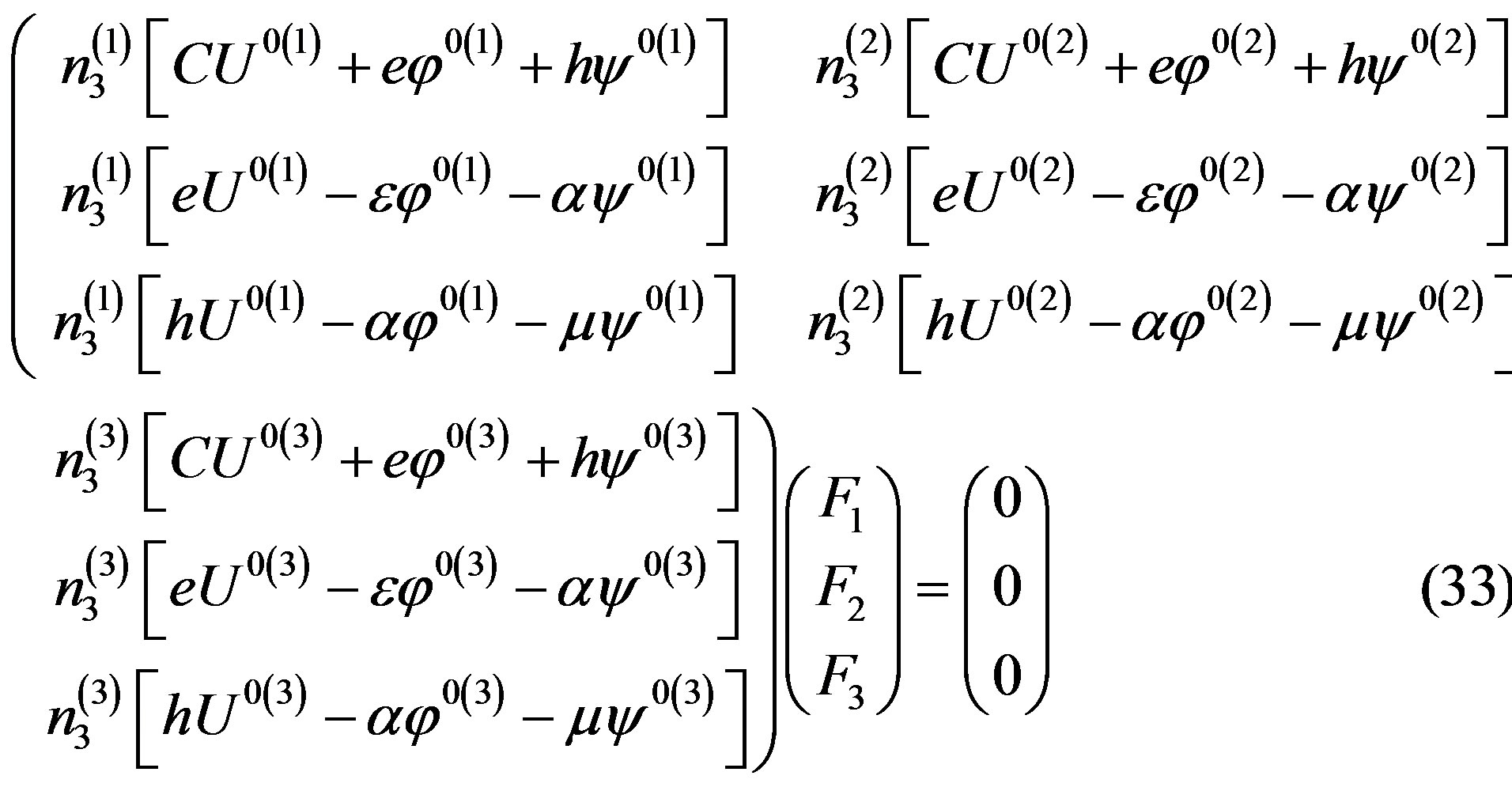
Following the theoretical treatments done in book [20], the utilization of these boundary conditions results in the following system of three homogeneous equations written in the matrix form:

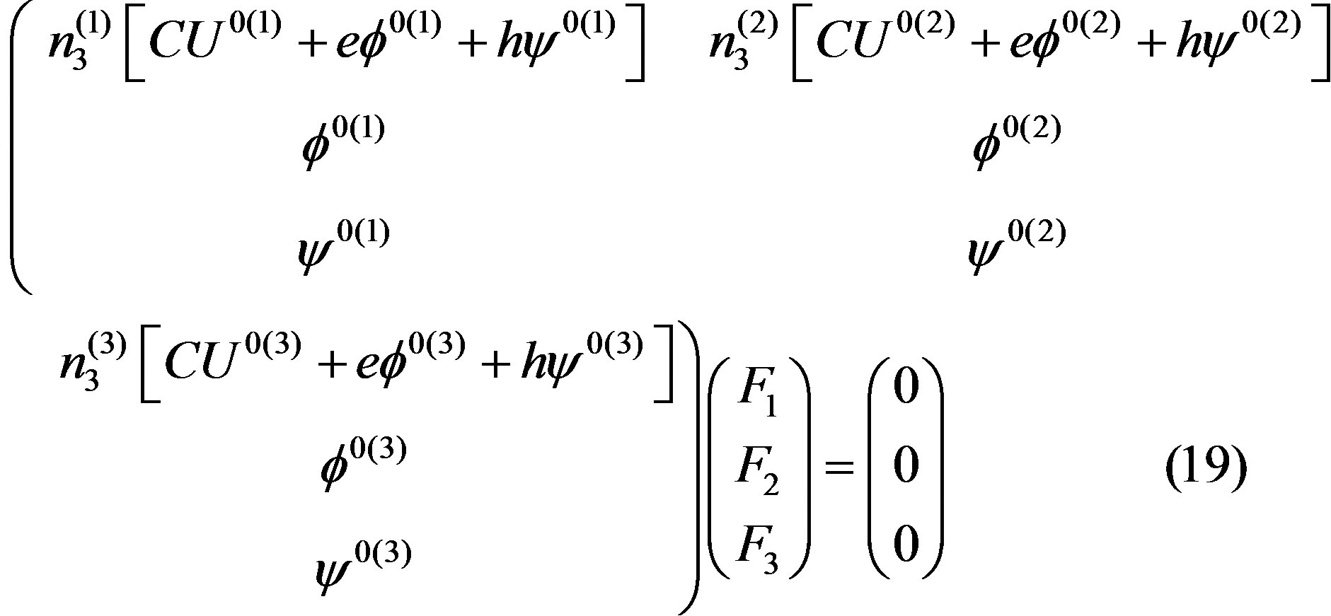
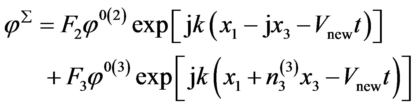
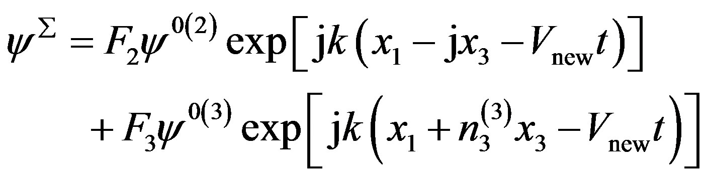
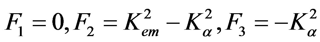
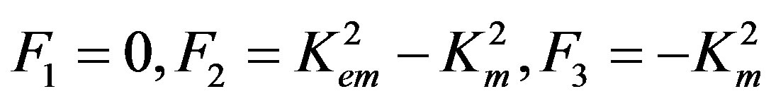
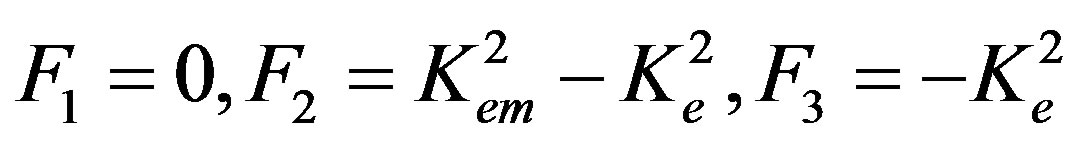
In Equations (19), F₁, F₂, and F₃ are the weight factors which must be determined. They are very important parameters. The complete mechanical displacement U^Σ, complete electrical potential φ^Σ, and complete magnetic potential ψ^Σ depend on them and can be written in the plane wave forms as follows:

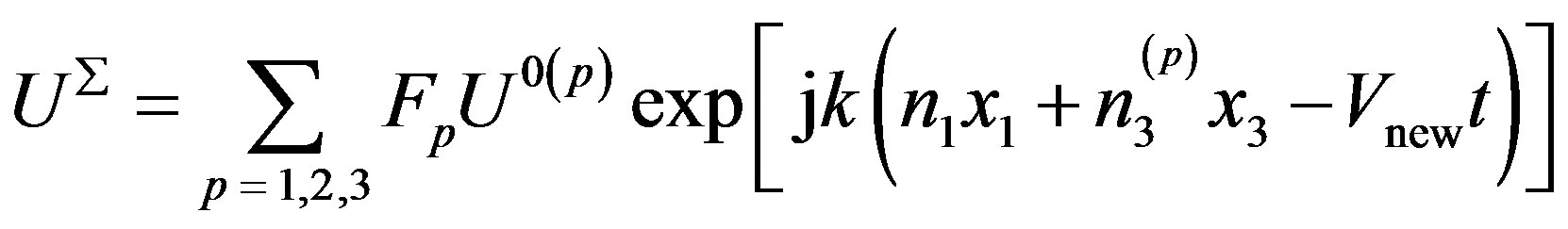(20)

(21)

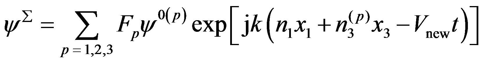(22)

where x₃ < 0 and V_new is defined by expression (8).

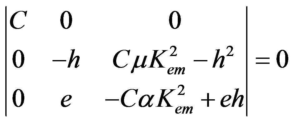
To determine the values of the weight factors, it is necessary to use in Equation (19) the eigenvalues and the corresponding eigenvector components. Exploiting them and the first set of the eigenvector components defined by expression (17), one can obtain the explicit form for the first third-order boundary-condition determinant (BCD3) of the coefficient matrix in Equation (19). It is as simple as follows:

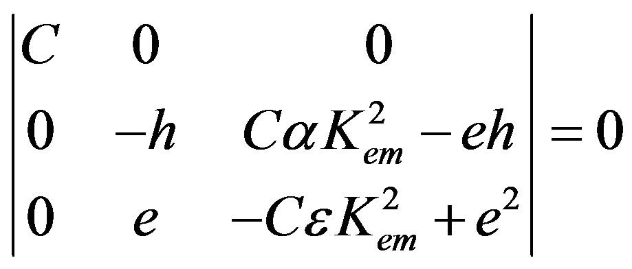(23)

Expanding it, one can obtain the following secular equation, in which only material constants are involved because the phase velocity V_ph was determined in Equation (8):

(24)

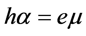
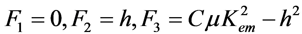
It is clearly seen in Equation (24) that the left-hand side is formed by two factors. Therefore, there are two possibilities to satisfy the equality in Equation (24) when either the first or second factor equals to zero. The equality to zero of the first factor leads to the following existence condition for the new wave propagation in the cubic piezoelectromagnetics:

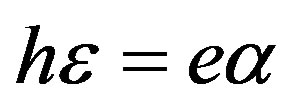(25)

For this condition, it is possible to find the explicit forms of the weight factors. Using Equations (19) and (23), one can check that the simplest forms are expressed as follows:

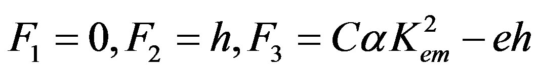(26)

In Equation (24), the equality to zero of the second factor representing the CMEMC K_em² defined by relation (9) is inappropriate here. This is true because n₃⁽³⁾(K_em² = 0) = n₃⁽²⁾, see formulae (14) and (16). In this case there are two equal eigenvalues which give the same sets of the eigenvector components. This situation was also mentioned in the previous section. As a result, F₂ = –F₃ together with F₁ = 0 will zero the complete displacements defined by formulae from (20) to (22). So, this possibility is excluded.

Therefore, the complete displacements defined by formulae from (20) to (22) represent those corresponding to the new wave propagation. These new wave can be called surface electromagnetic wave due to F₁ = 0 in expression (26) and U⁰⁽³⁾ = 0 (see expression (27) below) in expression (17) for condition (25). They then read:

(27)

(28)

(29)

where x₃ < 0 means that the new wave must damp towards the depth of the cubic piezoelectromagnetics. In expressions from (27) to (29), the speed of the new wave V_new is defined by expression (8). Using definition (17) for U⁰⁽³⁾ and existence condition (25), it is flagrantly seen in Equation (27) that the complete mechanical displacement U^Σ is equal to zero.

This fact can be understood by the way that the wave propagation specifics exhibits a compensative character, namely U⁰⁽³⁾ = (hε – eα)K_em² = 0 (17) due to hε = eα (25). This can mean that this slow wave is truly acoustic and the piezoelectromagnetic properties can compensate the mechanical ones resulting in zero value of the mechanical displacement during the wave propagation. Indeed, this slow wave propagates with the speed slightly above the SH-BAW speed V_tem. It is well-known that acoustic wave speeds including the V_tem and V_new are approximately five orders slower than the speed of the electromagnetic wave propagating in a bulk solid. It is defined by the following relation: V² = (εµ)^–1. This extreme slowness of the new wave illustrates that some connection with the mechanical displacement is conserved. Therefore, the new wave can be called the surface acoustic magnetoelectric wave to illuminate that this wave relates to an acoustic branch, but not an optic branch.

This new electromagnetic wave can be also called the surface acoustic-phonon polariton (SAPP) to distinguish from the surface optic-phonon polaritons (SOPPs). The SOPPs [34] are well-known and the SOPPs on crystal substrates have applications in microscopy, biosensing, and photonics. The SOPPs represent electromagnetic surface modes formed by the strong coupling of light and optical phonons in polar crystals, and are generally excited using IR or THz radiation. Generation and control of the SOPPs are essential for realizing novel applications in microscopy, data storage, thermal emission, or in the field of metamaterials. However, a comparatively little attention is still focused on the SOPPs despite certain advantages including their ability to be generated in a wide spectral range, from IR to THz wavelengths at the surface of a large variety of semiconductors, insulators, and ferroelectrics [34]. It was also mentioned in Ref. [35] that surface electromagnetic effects could enhance the efficiency of numerous physical and chemical processes [36], as these effects lead to an increase of the electromagnetic fields at the surface, giving rise to an improved experimental sensitivity.

Utilizing the second set of the eigenvector components defined by expression (18) for the third eigenvalue, the second BCD3 reads:

(30)

Expanding this BCD3, the following second existence condition of the wave propagation in the cubic piezoelectromagnetics can be revealed:

(31)

Therefore, the explicit forms of the weight factors are as follows:

(32)

For this second case, the complete displacements of the new wave can be written in the same forms defined by formulae from (27) to (29), where the weight factor F₃ from definitions (32) and the second set of the eigenvector components given in expression (18) must be used. It is thought that it is vital to treat the other possible sets of the boundary conditions for comparison.

2.2. σ₃₂ = 0, D = 0, and B = 0

Using this set of the mechanical, electrical, and magnetic boundary conditions, it is possible to write the following homogeneous equations [20]:

The matrix BCD3 representing a number can be then written in the following simplified form, using Equation (17):

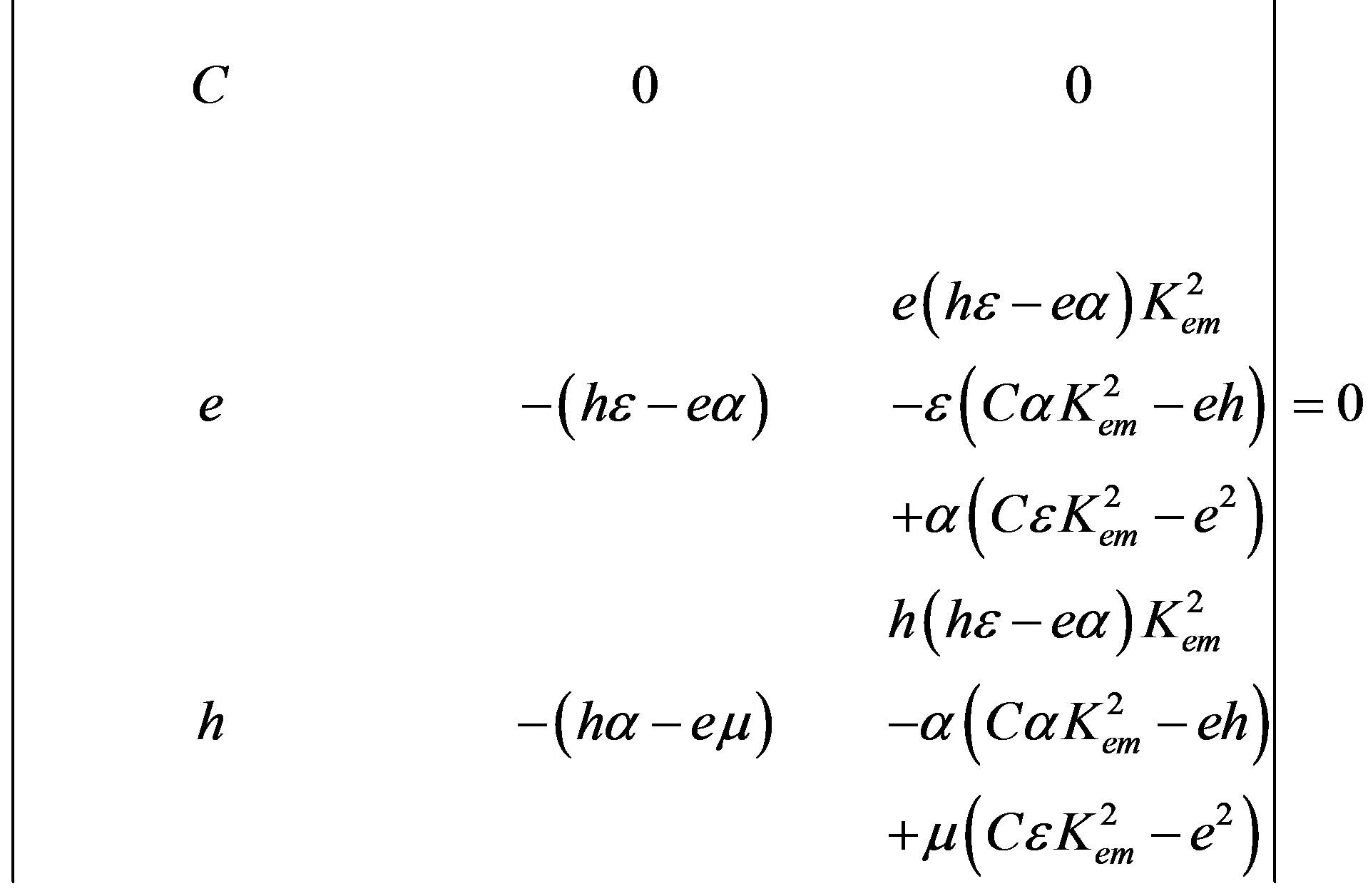(34)

The BCD3 in Equation (34) can be readily reduced to the following determinant:

(35)

It is clearly seen in the first row of determinant (35) that the determinant equals to zero when (25). This coincides with the result obtained in Subsection 2.1. Using the second row of the determinant, the explicit forms of the weight factors are written as follows:

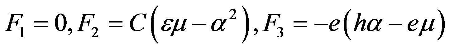(36)

The weight factors are used in equations from (27) to (29), too. It is also necessary to mention the second solution for Equation (35). This is as follows:

(37)

This second solution (37) looks like unreal or it is hard to realize it. However, it is thought that it is useful to record any solution to have a more complete picture of the problem of wave propagation.

Using eigenvector components (18) for Equations (33), one can get the following BCD3:

(38)

It is obvious that one can transform determinant (38) by the same way, see the transformations of determinant (35) written above. It was found that determinant (38) equals to zero when (31). This also coincides with the result obtained in Subsection 2.1. There is also the second solution which coincides with expression (37). For the case of the first solution for Equation (38), the explicit forms of the weight factors read:

(39)

The values of weight factors (39) are also utilized in equations from (27) to (29). Therefore, it is possible to state that the cases of the boundary conditions used in this and the previous subsections demonstrate the same results.

2.3. σ₃₂ = 0, φ = 0, and B = 0

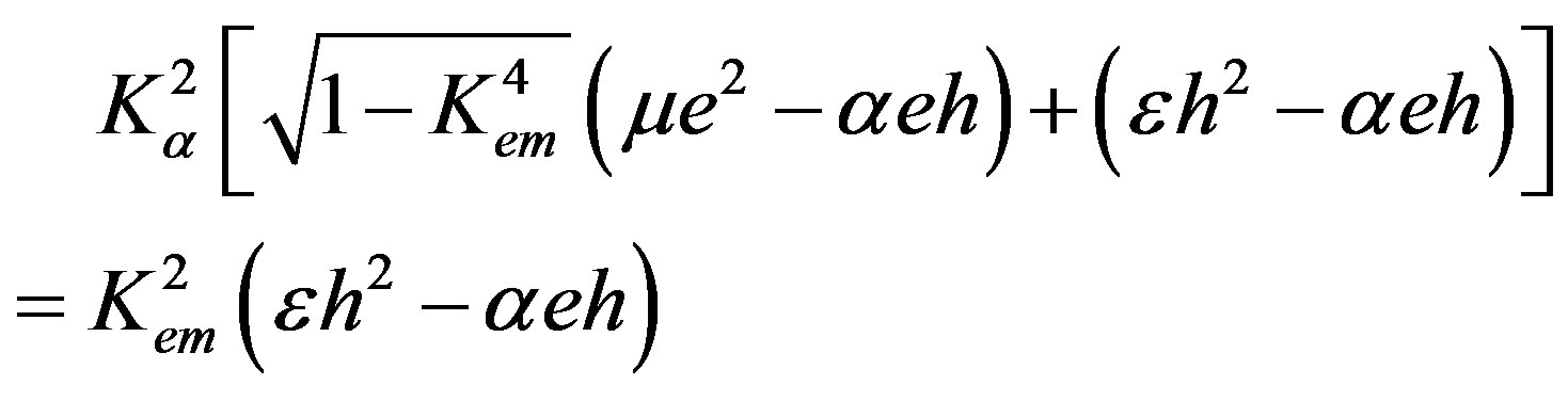
This is the case of the mechanically free (σ₃₂ = 0), electrically closed (φ = 0), and magnetically closed (B = 0) surface. It is obvious that this is the case when the electrical and magnetic boundary conditions are used from Subsections 2.1 and 2.2, respectively. Therefore, the reader can readily form the corresponding three homogeneous equations in the matrix form (this form can be also found in book [20]) similar to Equations (19) and (33). Also, the reader can use definitions (17) and (18) in order to get two different BCDs of the coefficient matrix. Using expression (17), it is possible to expand the corresponding first BCD3 and to obtain the following equation:

(40)

where the nondimensional value of K_α² was introduced in the recent book cited in Ref. [20], K_α² = eh/(Cα).

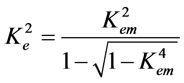
Equation (40) represents the existence condition for the new wave propagation in the case studied in this subsection. The new wave propagates with the speed defined by relation (8). It is evident that Equation (40) is very complicated. For small values of α, the value of K_α² can be very large. Therefore, it is necessary to cope with small values of the material constant h in order to have appropriate values of K_α², namely 0 < K_α² < 1 similar to 0 < K_em² < 1. It is clear that for small values of α and h, the value of K_em² is completely defined by the piezoelectric properties. This can be the case of the dominant piezoelectric phase. However, it is thought that this dominance is not obligatory in the case of a large value of α. Indeed, the value of K_em² can be large, but less than unity. Consequently, equality (40) can be fulfilled when the following occurs: K_α² → K_em² → K_e², where K_e² is called the coefficient of the electromechanical coupling (CEMC). It represents the well-known non-dimensional characteristic for a pure piezoelectrics and can also define the piezoelectric phase of a piezoelectromagnetics. It is defined by the following relation:

(41)

Also, it is possible to introduce the weight factors for this case in non-dimensional forms. They are written as follows:

(42)

Therefore, it is possible to state that existence condition (40) can give non-zero values of the complete mechanical displacement U^Σ in Equation (27). This means that for the mechanically free, electrically closed, and magnetically closed surface, the new surface wave can represent the new SH-SAW coupled with both the electrical and magnetic potentials.

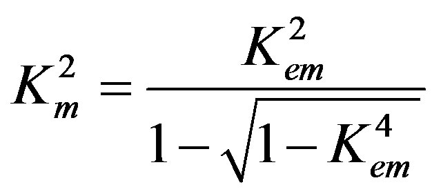
Using Equation (18), it is possible to form the second BCD3 for determination of the existence conditions of the new wave propagation for this set of the boundary conditions. It was found that three solutions (existence conditions) can exist in this case. The first existence condition coincides with that revealed in formula (31):. The second solution such as K_em² = 0 is inappropriate because it gives two equal eigenvalues n₃⁽²⁾ = n₃⁽³⁾ = –j. This was discussed above. The third existence condition is complicated. This is a limit case and gives K_m² → K_em² → 1. However, K_em² = 1 is also unsuitable because it gives V_new = V_tem. This was also discussed above. The limit condition reads:

(43)

where K_m² is called the coefficient of the magnetomechanical coupling (CMMC). It represents the well-known non-dimensional characteristic for a pure piezomagnetics and can also define the piezomagnetic phase of a piezoelectromagnetics. It is defined by

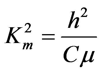(44)

The weight factors can be then written in nondimensional forms as follows:

(45)

2.4. σ₃₂ = 0, D = 0, and ψ = 0

In this case of the mechanically free (σ₃₂ = 0), electrically open (D = 0), and magnetically open (ψ = 0) surface, two different sets of eigenvector components (17) and (18) must be also applied. It is obvious that this is the case when the electrical and magnetic boundary conditions can be borrowed from Subsections 2.2 and 2.1, respectively. Indeed, the reader can also form three homogeneous equations in the matrix form and expand the BCD3 of the coefficient matrix by the way demonstrated in Subsections 2.1 and 2.2. Using definition (17) to form the first BCD3 and expanding the BCD3, one can also obtain three limit existence conditions. All of them are unsuitable similar to those for the second BCD3 from Subsection 2.3. They read: (25), K_em² = 0, and K_e² → K_em² → 1. Indeed, K_em² = 1 is inapt because it gives the case of V_new = V_tem discussed above and results from the following limit condition:

(46)

Therefore, the weight factors are as follows:

(47)

Using definition (18) to form the second BCD3, one can find single suitable existence condition because the BCD3 can reduce to the following equality after expansion:

(48)

Existence condition (48) looks like existence condition (40) for the new wave propagation in the case of Subsection 2.3. In the case of this subsection, the new wave also propagates with the speed defined by relation (8). Indeed, for small values of α, the value of K_α² can be very large. Therefore, it is necessary to cope with small values of the material constant e in order to get the following: 0 < K_α² < 1 similar to 0 < K_em² < 1. It is lucid that for very small values of α and e, the value of K_em² is completely defined by the piezomagnetic properties: The piezomagnetic phase can be dominant and this dominance is not obligatory in the case of a large value of α. Indeed, the value of K_em² can be large, but less than unity. Consequently, Equality (48) can be also fulfilled when the following occurs: K_α² → K_em² → K_m². It is expected that in the case of large values of α and e, Equality (48) with K_α² < 1 can be also true for suitable values of all the material constants of the cubic piezoelectromagnetics. Finally, it is indispensable to mention that the weight factors for this case are those introduced in Equation (42) in the nondimensional forms.

3. Discussion

These theoretical investigations carried out above soundly demonstrated that an additional surface wave can propagate in direction [101] in the cubic piezoelectromagnetics. This new wave has a unique propagation characteristic such as follows: Its speed is higher than the SH-BAW speed. This fact can relate this type of wave to leaky surface SH-waves. However, it is actually a surface wave. As a result, it is possible to state that in the cubic piezoelectromagnetics, nine different surface waves (including such SH-SAW as the surface BGM-wave) can propagate in the same suitable propagation direction, using different boundary conditions. For comparison, ten different SH-SAWs under application of the same possible boundary conditions can propagate in the transversely isotropic piezoelectromagnetic materials. It is worth noting that as soon as one will apply the theory developed in this work to the transversely isotropic piezoelectromagnetics to discover any SH-LSAW, one can possibly find that in such materials the suitable propagation speed is equal to zero. This can mean that such SH-SAW cannot be found in the transversely isotropic piezoelectromagnetics. However, it is possible that some types of leaky waves can exist in the materials.

Concerning the propagation of the new wave in the cubic piezoelectromagnetics, it is possible to briefly discuss the revealed existence conditions given by formulae (25) and (31) in the previous section. These obtained existence conditions are true for the applied boundary conditions of Subsection 2.1 such as the normal component of the stress tensor must vanish, φ = 0 and ψ = 0. Using the other boundary conditions in subsections from 2.2 and 2.4, one can find the other existence conditions which can be different from obtained Equalities (25) and (31). Also, the suitable existence conditions obtained in Subsections 2.3 and 2.4 can result in the fact that the new surface wave can become the new SH-SAW. It is worth noting that the wave speed defined by Formula (8) is the same for each suitable existence condition resulting in the possible propagation of the new surface electromagnetic wave or the new SH-SAW.

Indeed, existence Conditions (25) and (31) completely depend on the material constants of the cubic piezoelectromagnetics. The first condition defined by Equality (25), namely demonstrates that this case can be realized with suitable cubic piezoelectromagnetics which can have as large as possible values of the piezoelectric constant e and the electromagnetic constant α. Their typical values are as follows: from ~0.1 to ~10 C/m² and by about 10^–12 s/m, respectively. On the other hand, the values of the piezomagnetic coefficient h and dielectric permittivity constant ε must be small enough. The typical values of h are from ~1 to ~10³ Tesla and those for ε are ~10^{–10 F/m. It is possible to say that here the piezoelectric phase must be dominant. It is obvious that it is necessary to use suitable cubic piezoelectromagnetics with a very weak piezomagnetic phase for experimental investigations. It is possible that suitable values of h must be from ~10–3} to ~10^–5 Tesla or even less. It is thought that such small values of h can be also achieved in composites when a piezoelectric-phase matrix is used in which a weak piezomagnetic phase is properly added. Therefore, the experimental techniques for measurements of the material constant h must be improved because experimentalists frequently write zero instead of such small values of h.

Indeed, the values of all the material constants depend on the value of the applied magnetic or electric field. Therefore, one can deal with many parameters and it is possible to suggest that some material constants can depend stronger than the others. This can be different for different piezoelectromagnetics. Therefore, it is possible that a class of suitable piezoelectromagnetics can be formed. This activity can represent intensive experimental investigations in the future for decades. It is thought that some technical devices using such surface wave can be extremely sensitive (supersensors) because any infinitesimal change in the applied magnetic (or electric) field can cause a propagation problem for such surface wave. Therefore, the wave can vanish. As soon as propagation Condition (25) is restored, the wave can then propagate anew.

The second condition defined by Formula (31), namely also couples four material constants such as the piezoelectric e, piezomagnetic h, magnetic permeability µ, and electromagnetic α. Because the value of α is always very small, the value of h must be as large as possible and the values of e and µ must be as small as possible. It is obvious that the value of µ is restricted by the value of µ₀ for a vacuum. However, it is thought that there is no restriction to minimize the value of the piezoelectric constant e down to suitable very small values. Indeed, this class of cubic piezoelectromagnetics is for those with a dominant piezomagnetic phase. Therefore, it is very important to account measured very small value of the piezoelectric constant e, but not write zero instead. It is possible that such native cubic piezoelectromagnetics can exist. Also, it is thought that artificial composites can be readily created when a strong cubic piezomagnetics can be used as the suitable matrix to solute a very weak piezoelectric phase.

Also, it is possible to mention the other artificial materials which are well-known. They are metamaterials. These materials possess µ < 0 and ε < 0 resulting in εµ > 0. It is apparent that for such metamaterials, the value of the electromagnetic constants α should have a negative sign to satisfy the conditions written in Formulae (25) and (31). This theoretical work does not have a purpose to solidly demonstrate that Conditions (25) and (31) can be also true for some suitable metamaterials. Indeed, this is possible. Note that the metamaterials are new material and they are extensively studied concerning various applications. However, it is possible to review some recent papers concerning a variety of investigations of the metamaterials. Refs. [37,38] have reported their studies of left-handed artificial materials (metamaterials) in the frequency region from 1 THz to 100 THz, and even above [37]. The main problem of the experimental reports in Refs. [37-39] is the fact that they do not provide the complete set of material constants for investigated unique composites. Ref. [40] reported a study of piezoelectric-piezomagnetic multilayer with ε < 0 and μ < 0 in which dielectric polariton and magnetic polariton can be simultaneously created. Also, it was recently stated that phonon-polaritons in a form of a band-like structure can exist in piezomagnetic superlattices (PMSL) with periodically up and down polarized domain structures [41] in which the piezomagnetic coefficients are periodically modulated. Also, some theoretical approaches exist which use material constants with real and imaginary parts (complex numbers) to describe wave propagation in multi-layered structures [42]. Some works concerning the investigations of different metamaterials can be also found in Refs. [43,44]. It is noted that Ref. [44] deals with three-dimensional bulk metamaterials. Therefore, it is thought that SH-BAWs and SH-SAWs can be investigated in bulk metamaterials.

Also, it is necessary to state that this problem of the surface wave propagation discussed above in this work relates to the cubic piezoelectromagnetics (two-phase materials with the cubic symmetry) but not to the pure piezomagnetics or pure piezoelectrics possessing the cubic symmetry. These single-phase materials were theoretically studied in Refs. [21] and [22], correspondingly. That is true because the piezoelectric constant e vanishes in the case of pure piezomagnetics. As a result, existence Condition (25) such as and (31) such as cannot be fulfilled because of h = 0 and e ≠ 0 in the case of pure piezoelectrics or h ≠ 0 and e = 0 in the case of pure piezomagnetics. Indeed, one can note that it is possible to require α = 0 for both the cases mentioned above to fulfill Equalities (25) and (31). However, one will cope here with zeroes on both sides of Equalities (25) and (31). For that reason, it is necessary to work with non-zero values of the material constants: h ≠ 0, e ≠ 0, and α ≠ 0.

4. Conclusion

This report represents the theoretical description of the new wave propagation in direction [101] in the cubic piezoelectromagnetics. The new wave can propagate with the speed higher than that for the SH-BAW coupled with both the electrical and magnetic potentials when 0 < K_em² < 1. The existence conditions for the new wave propagation were revealed. These conditions can be complicated and are coupled with the values of the material constants of the cubic piezoelectromagnetics. It is wellknown that the value of the electromagnetic constant α is very small. Therefore, to satisfy some existence conditions, the two-phase (composite) material must possess the material properties resulting in the domination of the piezoelectric phase with a significantly weaker piezomagnetic phase or the domination of the piezomagnetic phase with a significantly weaker piezoelectric phase. Indeed, if the suitable existence conditions obtained in subsections from 2.1 to 2.4 can be realized, the new wave can propagate. Using suitable Condition (40) or (48), it is expected that the new wave can also represent the new SH-SAW. It is also expected that any infinitesimal perturbation of the medium surface along the new wave propagation way can cause a dramatic attenuation of such wave. This can be used in creation of various technical devices, for instance, supersensors.

5. Acknowledgements

The author thanks to the referee and the members of the Editorial Board for a large interest in my theoretical work.

REFERENCES

- J. van Suchtelen, “Product Properties: A New Application of Composite Materials,” Philips Research Reports, Vol. 27, No. 1, 1972, pp. 28-37.
- J. van den Boomgaard, D. R. Terrell, R. A. J. Born and H. F. J. I. Giller, “In-Situ Grown Eutectic Magneto Electric Composite-Material. 1. Composition and Unidirectional Solidification,” Journal of Materials Science, Vol. 9, No. 10, 1974, pp. 1705-1709.
- A. M. J. G. van Run, D. R. Terrell and J. H. Scholing, “In-Situ Grown Eutectic Magnetoelectric Composite-Material. 2. Physical Properties,” Journal of Materials Science, Vol. 9, No. 10, 1974, pp. 1710-1714.
- J. van den Boomgaard, A. M. J. G. van Run and J. van Suchtelen, “Piezoelectric-Piezomagnetic Composites with Magnetoelectric Effect,” Ferroelectrics, Vol. 14, No. 1, 1976, pp. 727-728. doi:10.1080/00150197608236711
- V. E. Wood and A. E. Austin, “Possible Applications Magnetoelectric,” In: A. J. Freeman and H. Schmid, Eds., Magnetoelectric Interaction Phenomena in Crystals, Gordon and Breach Science Publishers, Newark, 1975, pp. 181-194.
- G. Srinivasan, “Magnetoelectric Composites,” Annual Review of Materials Research, Vol. 40, 2010, pp. 153-178. doi:10.1146/annurev-matsci-070909-104459
- Ü. Özgür, Ya. Alivov and H. Morkoç, “Microwave Ferrites, Part 2: Passive Components and Electrical Tuning,” Journal of Materials Science: Materials in Electronics, Vol. 20, No. 10, 2009, pp. 911-952. doi:10.1007/s10854-009-9924-1
- J. Zhai, Z.-P. Xing, Sh.-X. Dong, J.-F. Li and D. Viehland, “Magnetoelectric Laminate Composites: An Overview,” Journal of the American Ceramic Society, Vol. 91, No. 2, 2008, pp. 351-358. doi:10.1111/j.1551-2916.2008.02259.x
- M. Fiebig, “Revival of the Magnetoelectric Effect,” Journal of Physics D: Applied Physics, Vol. 38, No. 8, 2005, pp. R123-R152. doi:10.1088/0022-3727/38/8/R01
- W. Eerenstein, N. D. Mathur and J. F. Scott, “Multiferroic and Magnetoelectric Materials,” Nature, Vol. 442, 2006, pp. 759-765. doi:10.1038/nature05023
- M. Bichurin, V. Petrov, A. Zakharov, D. Kovalenko, S. Ch. Yang, D. Maurya, V. Bedekar and Sh. Priya, “Magnetoelectric Interactions in Lead-Based and Lead-Free Composites,” Materials, Vol. 2011, No. 4, 2011, pp. 651- 702. doi:10.3390/ma4040651
- G. A. Smolenskii and I. E. Chupis, “Ferroelectromagnets,” Soviet Physics Uspekhi (Uspekhi Phizicheskikh Nauk, Moscow), Vol. 25, No. 7, 1982, p. 475.
- W. Cheong and M. Mostovoy, “Multiferroics: A Magnetic Twist for Ferroelectricity,” Nature Materials, Vol. 6, 2007, pp. 13-20. doi:10.1038/nmat1804
- R. Ramesh and N. A. Spaldin, “Multiferroics: Progress and Prospects in Thin Films,” Nature Materials, Vol. 6, 2007, pp. 21-29. doi:10.1038/nmat1805
- T. Kimura, “Spiral Magnets as Magnetoelectrics,” Annual Review of Materials Research, Vol. 37, 2007, pp. 387- 413. doi:10.1146/annurev.matsci.37.052506.084259
- A. Melkumyan, “Twelve Shear Surface Waves Guided by Clamped/Free Boundaries in Magneto-Electro-Elastic Materials,” International Journal of Solids and Structures, Vol. 44, 2007, pp. 3594-3599. doi:10.1016/j.ijsolstr.2006.09.016
- A. A. Zakharenko, “Propagation of Seven New SH-SAWs in Piezoelectromagnetics of Class 6 mm,” LAP LAMBERT Academic Publishing GmbH & Co. KG, Saarbruecken-Krasnoyarsk, 2010, p. 84.
- J. L. Bleustein, “A New Surface Wave in Piezoelectric Materials,” Applied Physics Letters, Vol. 13, No. 12, 1968, pp. 412-413. doi:10.1063/1.1652495
- Yu. V. Gulyaev, “Electroacoustic Surface Waves in Solids,” Soviet Physics Journal of Experimental and Theoretical Physics Letters, Vol. 9, 1969, pp. 37-38.
- A. A. Zakharenko, “Seven New SH-SAWs in Cubic Piezoelectromagnetics,” LAP LAMBERT Academic Publishing GmbH & Co. KG, Saarbruecken-Krasnoyarsk, 2011, p. 172.
- A. A. Zakharenko, “First Evidence of Surface SH-Wave Propagation in Cubic Piezomagnetics,” Journal of Electromagnetic Analysis and Applications, Vol. 2, No. 5, 2010, pp. 287-296.
- A. A. Zakharenko, “New Solutions of Shear Waves in Piezoelectric Cubic Crystals,” Journal of Zhejiang University SCIENCE A, Vol. 8, No. 4, 2007, pp. 669-674. doi:10.1631/jzus.2007.A0669
- R. Ribichini, F. Cegla, P. B. Nagy and P. Cawley, “Quantitative Modeling of the Transduction of Electromagnetic Acoustic Transducers Operating on Ferromagnetic Media,” IEEE Transactions on Ultrasonics, Ferroelectrics, and Frequency Control, Vol. 57, No. 12, 2010, pp. 2808- 2817. doi:10.1109/TUFFC.2010.1754
- R. B. Thompson, “Physical Principles of Measurements with EMAT Transducers,” In: W. P. Mason and R. N. Thurston, Eds., Physical Acoustics, Academic Press, New York, Vol. 19, 1990, pp. 157-200.
- M. Hirao and H. Ogi, “EMATs for Science and Industry: Noncontacting Ultrasonic Measurements,” Kluwer Academic, Boston, 2003.
- Sh. Kakio, T. Yamaguchi and Ya. Nakagawa, “Leaky Surface Acoustic Waves on Langasite with Thin Dielectric Films,” Japanese Journal of Applied Physics, Vol. 41, No. 5B, 2002, pp. 3494-3497.
- H. Zhang, M. Murota and Ya. Shimizu, “Characteristics of Longitudinal Leaky Surface Waves Propagating on La3Ga5SiO14 Substrate,” Japanese Journal of Applied Physics, Vol. 40, No. 5B, 2001, pp. 3755-3758.
- T. Sato, M. Murota and Ya. Shimizu, “Characteristics of Rayleigh and Leaky Surface Acoustic Wave Propagating on a La3Ga5SiO14 Substrate,” Japanese Journal of Applied Physics, Vol. 37, No. 5B, 1998, pp. 2914-2917.
- M. Kadota, J. Nakanishi, T. Kitamura and M. Kumatoriya, “Properties of Leaky, Leaky Pseudo, and Rayleigh Surface Acoustic Waves on Various Rotated Y-Cut Langasite Crystal Substrates,” Japanese Journal of Applied Physics, Vol. 38, No. 5B, 1999, pp. 3288-3292.
- K. Hasegawa and M. Koshiba, “Coupled-Mode Equations for Interdigital Transducers for Leaky Surface Acoustic Waves,” Japanese Journal of Applied Physics, Vol. 42, No. 5B, 2003, pp. 3157-3160.
- R. Nakagawa, T. Yamada, T. Omori, K.-Y. Hashimoto and M. Yamaguchi, “Analysis of Excitation and Propagation Characteristics of Leaky Modes in Surface Acoustic Wave Waveguides,” Japanese Journal of Applied Physics, Vol. 41, No. 5B, 2002, pp. 3460-3164.
- V. E. Lyamov, “Polarization Effects and Interaction Anisotropy of Acoustic Waves in Crystals,” MSU Publishing, Moscow, 1983, p. 224.
- V. I. Al’shits, A. N. Darinskii and J. Lothe, “On the Existence of Surface Waves in Half-infinite Anisotropic Elastic Media with Piezoelectric and Piezomagnetic Properties,” Wave Motion, Vol. 16, No. 3, 1992, pp. 265-283. doi:10.1016/0165-2125(92)90033-X
- A. J. Huber, B. Deutsch, L. Novotny and R. Hillenbrand, “Focusing on Surface Phonon Polaritons,” Applied Physics Letters, Vol. 92, No. 20, 2008, p. 3.
- I. Minin and O. Minin, “3D Diffractive Focusing THz of In-Plane Surface Plasmon Polariton Waves,” Journal of Electromagnetic Analysis & Applications, Vol. 2, 2010, pp. 116-119.
- G. C. Schatz and R. P. van Duyne, “Electromagnetic Mechanism of Surface-Enhanced Spectroscopy,” Wiley, New York, 2002.
- A. Ishikawa, T. Tanaka and S. Kawata, “Negative Magnetic Permeability in the Visible Light Region,” Physical Review Letters, Vol. 95, No. 23, 2005, p. 4.
- T. F. Gundogdu, I. Tsiapa, A. Kostopoulos, G. Konstantinidis, N. Katsarakis, R. S. Penciu, M. Kafesaki, E. N. Economou, Th. Koschny and C. M. Soukoulis, “Experimental Demonstration of Negative Magnetic Permeability in the Far-Infrared Frequency Regime,” Applied Physics Letters, Vol. 89, No. 8, 2006, p. 3.
- S. T. Chui, W. H. Wang, L. Zhou and Z. F. Lin, “Longitudinal Elliptically Polarized Electromagnetic Waves in Off-Diagonal Magneto Electric Split-Ring Composites,” Journal of Physics: Condensed Matter, Vol. 21, No. 29, 2009, p. 4.
- H. Liu, S. N. Zhu, Y. Y. Zhu, Y. F. Chen, N. B. Ming and X. Zhang, “Piezoelectric-Piezomagnetic Multilayer with Simultaneously Negative Permeability and Permittivity,” Applied Physics Letters, Vol. 86, No. 10, 2005, p. 3.
- Zh. X. Liu and W. Y. Wang, “Study of the Phonon-Polaritons in Piezomagnetic Superlattices Using a Generalized Transfer Matrix Method,” Journal of Physics: Condensed Matter, Vol. 18, No. 39, 2006, pp. 9083-9092. doi:10.1088/0953-8984/18/39/034
- C. Potel, S. Devolder, A. Ur-Rehman, J.-F. Belleval, J.-M. Gherbezza, O. Leroy and M. Wevers, “Experimental Verification of the Theory of Multilayered Rayleigh Waves,” Journal of Applied Physics, Vol. 86, No. 2, 1999, pp. 1128-1135. doi:10.1063/1.370854
- A. M. Shuvaev, S. Engelbrecht, M. Wunderlich, A. Schneider and A. Pimenov, “Strong Dynamic Magnetoelectric Coupling in Metamaterial,” The European Physical Journal B, Vol. 79, No. 2, 2011, pp. 163-167. doi:10.1140/epjb/e2010-10493-1
- W. T. Chen, Ch. J. Chen, P. Ch. Wu, Sh. Sun, L. Zhou, G.-Y. Guo, Ch. T. Hsiao, K.-Y. Yang, N. I. Zheludev and D. P. Tsai, “Optical Magnetic Response in Three-Dimensional Metamaterial of Upright Plasmonic Metamolecules,” Optics Express, Vol. 19, No. 13, 2011, pp. 12837- 12842. doi:10.1364/OE.19.012837