Theoretical Economics Letters
Vol.2 No.1(2012), Article ID:17348,6 pages DOI:10.4236/tel.2012.21002
Time Representation in Economics
EPEE (Centre d’Etudes des Politiques Economiques de l’Université d’Evry), University of Evry, Evry, France
Email: {stefano.bosi, lionel.ragot}@univ-evry.fr
Received October 31, 2011; revised November 27, 2011; accepted December 5, 2011
Keywords: Discretization; Growth
ABSTRACT
In this paper, we study general polynomial discretizations in backward and forward looking, and the preservation of stability properties. We apply these results to the Ramsey model [1]. Its discrete-time version is a hybrid discretizations of a backward-looking budget constraint and a forward-looking Euler equation. Saddle-path stability is a robust property under discretization.
1. Discretizations
Continuous-time systems can be approximated by discretetime systems. In the spirit of Krivine, Lesne and Treiner [2], we bridge continuous and discrete-time dynamics through general polynomial discretizations.
Discretizations can differ according to the step, the order and the direction of discretization. The step gives the length of the period in discrete time. The order is that of the Taylor expansion of a continuous-time model. The direction depends on the backward or forward-looking nature of this Taylor expansion. A hybrid discretization mixes backward and forward-looking approximations.
We want to show that the steady state is invariant to the step, the order and the direction of discretization and its continuous-time stability properties (sink, saddle, source) are preserved under a sufficiently small discretization step in any case (backward, forward or hybrid).
Instead of considering a continuous variable t and the corresponding position  determined by an m-dimensional system of ordinary differential equations:
  where
where  jointly with the initial condition
  let us pick up a regular sequence of time values:
 where h is a (possibly small) positive constant (discretization step), and the associated values:
 .
.
The path from  to
to  can be reconstructed component by component through an appropriate integration of
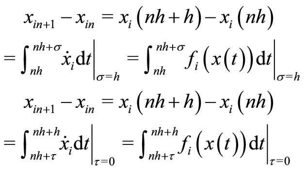
 . Focusing on the ith component of the vector
 , we can integrate the time derivative on the right or on the left to obtain, respectively,
with . Defining
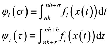
we get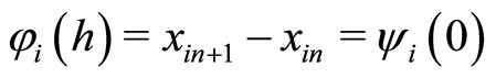 .
.
A discretization is an approximation of  (
( ) through a simpler function evaluated at
  (
( ). The Euler-Taylor discretization is a polynomial approximation. Assuming that
  and considering the qth order polynomial, we obtain a backward or a forward-looking discretization:
 (1)
(1)
 (2)
(2)
because . A discretization is said to be hybrid if (1) holds for some components of the vector x and (2) holds for the others.
Setting , we obtain from (1) and (2) a first-order discretization:
that is
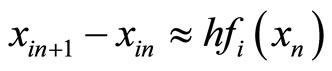 (3)
(3)
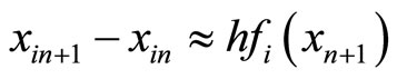 (4)
(4)
where the subscript i denotes the ith component of the vector.
Equation (3) (respectively, (4)) constitutes a backwardlooking (forward-looking) discretization, because the variation  depends on the past value
  (future value
 ) on the right-hand side. Equation (3) is the classical Euler discretization. In economics, forward-looking discretizations are of interest because agents behave according to their expectations.
The sequences  are approximations of the true sequence
 , exact solution to system
 : the smaller h, the more accurate the representation.
Higher-order discretizations are also possible. Let us discretize the continuous-time dynamical system  with
with  by second-order Taylor polynomials, that is approximate the ith component of
  with a quadratic form. Using (1) and (2), we obtain in backward and forward-looking, respectively:
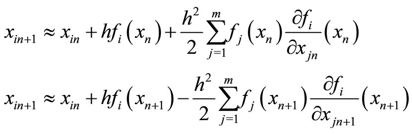
where the subscript i denotes the ith component of the vector.
If f is an analytic function, infinite-order backward or forward discretizations converge exactly to  and (1) and (2) now hold with equality:
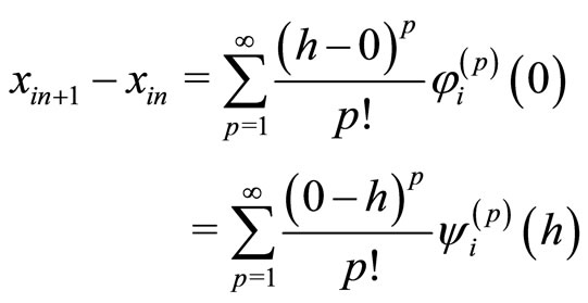
In this case, the Taylor polynomials become a convergent series and the discretized dynamics represent exactly the continuous-time system whatever the step h.
In general, a discretization is a closer approximation of a continuous-time system when the step h is smaller or the order of discretization q higher. The dynamic properties of a continuous-time system can be preserved lowering h or increasing q.
2. Dynamic Equivalence
To compare continuous-time and discrete-time system, we study approximations in a neighborhood of the steady state and focus on the persistence of local stability properties.
Focus first on the steady state. The system  and its discrete-time approximation
 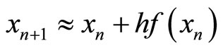 have the same steady state. Indeed, in both the cases, we require
  (respectively,
  and
and ). We further notice that the system of m equations
  neither depends on the discretization degree h nor on the discretization method (forward or backward-looking). Therefore, the steady state is invariant to discretization.
Focus now on the stability properties. Are they preserved under discretization in a neighborhood of the steady state?
Without loss of generality, we consider two-dimensional dynamics. In the spirit of Samuelson [3], we can represent the stability properties in the plane of trace T and determinant D of the Jacobian matrix J of the system evaluated at the steady state.
In the following, the subscripts  and 1 will denote variables in continuous or discrete time respectively.
1) In continuous time, stability depends on the real part of these eigenvalues. If both the real parts are negative (positive), the steady state is a sink (source) (in this case, the trace of  is negative (positive) and the determinant of
  is positive (positive)). If the signs of the real parts are different, the eigenvalues are real and the steady state is a saddle point (in this case, the determinant is negative).
2) In discrete time, the modulus of an eigenvalue  matters. When
  (
( ) the eigenvalue is inside (outside) the unit circle. If both the eigenvalues are inside (outside) the unit circle, the steady state is a sink (source). If one is inside and the other outside the unit circle, the steady state is a saddle point.
We can evaluate the characteristic polynomial

at –1 and 1. Focus on the  -plane. Along the line
 , one eigenvalue is equal to 1 because
  Along the line
 , one eigenvalue is equal to –1 because
  On the segment defined by
  and
and , the two eigenvalues are nonreal and conjugate with unit modulus. Consider first the points that neither belong to these lines nor to the segment. Inside the triangle defined by
  and
and  the steady state is a sink. It is a saddle point if
  lies on the left sides of both the lines
  and
and , or on the right sides of both of these lines (
 ). It is a source otherwise.
At least, a two-dimensional system is required to study the three cases (sink, saddle and source) together and to consider hybrid discretizations. Without loss of generality, we linearize the following system of ordinary differential equations
 (5)
(5)
Local dynamics around the steady state are represented by the Jacobian matrix  evaluated at the steady state (
 ).
).
We focus on first-order discretizations, but our equivalence results hold also for higher-order discretizations (see Bosi and Ragot [4]).
2.1. Backward-Looking Discretizations
We linearize the backward-looking discretization
 (6)
(6)
of the system (5) around the common steady state  and we obtain
 , where I and
  are the two-dimensional identity matrix and Jacobian matrix of system (6). We observe that
  depends on the steady state x which, in turn, does not depend on h. Then,
  depends only linearly on h.
As above, let us denote the trace and determinant of  and
and  by
by  and
and  respectively. The characteristic polynomial in discrete time is given by
 , where
 (7)
(7)
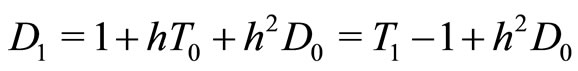 (8)
(8)
There are three critical values of the discretization step that determine the intervals of equivalence between the continuous and the discrete-time dynamics:
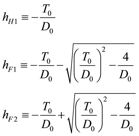
Proposition 1 Consider .
.
1) Let the steady state be a sink in continuous time (Figure 1).
1.1) If , then the steady state is a sink in discrete time if
  and a source if
 .
.
1.2) If  then the steady state is a sink if
 , a saddle if
 and source if
 .
.
2) If the steady state is a saddle in continuous time, then the steady state is a saddle in discrete time if  and source if
  (Figure 2).
3) If the steady state is a source in continuous time, then the source property is preserved whatever  (Figure 3).
The system generically undergoes a Hopf bifurcation at  and flip bifurcations at
 ,
, .
.
Proof From (7) and (8), it is possible to plot a curve  for each one of these different cases:
  given
given .
.
1) Assume that the steady state is a sink in continuous time: . According to (8),
 . Focus on two cases: (1.1)
  and (1.2)
 .
.
1.1) If  then always
  that is
  So, the steady state is a sink if
 , that is if
 , and a source if
 . This case corresponds to the upper parabola in Figure 1. Increasing h away from zero means moving away from the point where
 , along the parabola.

Figure 1. sink in continuous time.
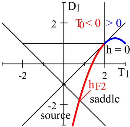
Figure 2. saddle in continuous time.
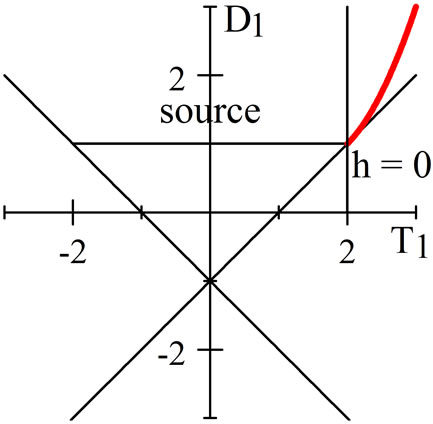
Figure 3. source in continuous time.
1.2) If  then
then  if and only if
 . In addition,
  if and only if
 . We notice also that
 . Then, the steady state is a sink if
 , a saddle if
  and a source if
 . This case corresponds to the lower parabola in Figure 1.
2) Assume now that the steady state is a saddle in continuous time:  According to (8),
  We observe that
  and that
  if and only if
  Thus, the steady state is a saddle if
  and a source if
  If
If  (
( )the curve
  is represented by the leftward (rightward) branch of parabola in Figure 2.
3) Assume now that the steady state is a source in continuous time:  and
and . (7) and (8) imply
  and
and  for every
 . Therefore the source property is preserved whatever
 . The branch of parabola in Figure 3 represents this case.
Corollary 2 (topological equivalence in backward looking) In any case of Proposition 1, there exists a nonempty interval  for the discretization step h where the stability properties of the continuous-time system are preserved.
Proof Straightforward. Simply observe that, in the case (3), .
.
2.2. Forward-Looking Discretizations
We linearize now the forward-looking discretization
 (9)
(9)
of system (5) around the common steady state  to obtain
Differently from the previous case, the Jacobian matrix of system (9)  is no longer linear in h. The trace and the determinant of
  are now given by
As above, we set three critical values: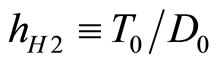 ,
,
Proposition 3 Consider .
.
1) If the steady state is a sink in continuous time, then the sink property is preserved in discrete time whatever .
.
2) Let the steady state be a saddle in continuous time.
2.1) If , then the steady state is a saddle.
2.2) If , then the steady state is a saddle if
  and a sink if
 .
.
3) Let the steady state be a source in continuous time.
3.1) Let . If
. If , then the source property is preserved whatever
  If
If , then the steady state is a source if
  or
or , and a saddle if
 .
.
3.2) Let . If
. If , then the steady state is a source if
  and a sink if
 . If
. If , then the steady state is a source if
  a saddle if
  and a sink if
 .
.
The system generically undergoes a Hopf bifurcation at  and flip bifurcations at
 ,
, .
.
Proof The proof is similar to that of Proposition 1. See Bosi and Ragot [4] for more details.
Corollary 4 (topological equivalence in forward looking) In every case of Proposition 3, there exists a nonempty interval  for the discretization step h where the stability properties of the continuous-time system are preserved.
Proof Straightforward. Simply observe that, in cases (1) and (2.1), . The same happens in the case (3.1) if
 .
.
2.3. Hybrid Discretizations
In economics, many higher-dimensional models require a hybrid discretization to recover the equivalence between discrete and continuous time, that is a mix of discretization in backward and forward looking. Without loss of generality, we consider a system where the first equation is discretized backward and the second one forward. Thus, the system of differential equations (5) becomes:
 (10)
(10)
 (11)
(11)
The steady state is invariant to the choice of time and to the type of discretization (backward/forward). The trace and the determinant of the Jacobian matrix  of the hybrid system (10)-(11) become
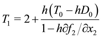 (12)
(12)
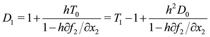 (13)
(13)
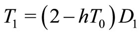
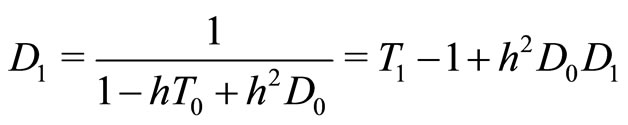
Notice that, in the particular case , (12) and (13) write
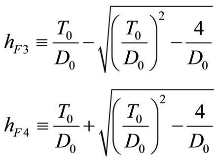
Let 
where .
.
Proposition 5 Consider .
.
1) Let .
.
1.1) If the steady state is a sink in continuous time, then the steady state in discrete time is a sink if  , and a saddle if
 .
.
1.2) Let the steady state be a saddle in continuous time.
1.2.1) If  or
or , then the steady state is a saddle point.
1.2.2) If  and
and , then the steady state is a saddle if
  or
or , and a source if
 .
.
1.3) If the steady state is a source in continuous time, then the steady state is a source if  and a saddle if
 .
.
2) Let  with
with . All the previous cases hold, provided we restrict the analysis to the interval
 .
.
The system generically undergoes a Hopf bifurcation at  and a flip bifurcation at
 ,
, .
.
Proof The proof is similar to that of Proposition 1. See Bosi and Ragot [4] for more details.
Corollary 6 (topological equivalence in hybrid looking). In every case of Proposition 5, there exists a nonempty interval  for the discretization step h where the stability properties of the continuous-time system are preserved.
Proof Straightforward. Simply observe that, in the case (1.2.1), .
.
3. Ramsey Model
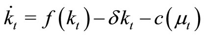
In the seminal Ramsey [1], the planner maximizes the undiscounted dynastic utility: , under a resource constraint
  where
where  and
and  denote the individual capital and consumption. The initial endowment
  is given.
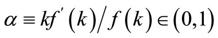
The intensive production function  is strictly increasing and strictly concave in the capital intensity and satisfies the Inada conditions. The felicity
  is also strictly increasing and strictly concave in the consumption level. c denotes the bliss point, that is the steady state value of consumption:
  with
with .
.
The planner maximizes the Hamiltonian:
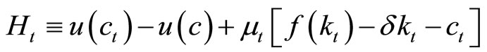
to find the first-order conditions:
 (14)
(14)
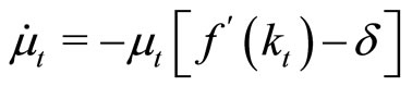 (15)
(15)
where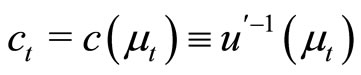 . The strict concavity of u ensures that
  is a well-defined function of the multiplier
 .
.
In discrete time, the planner maximizes 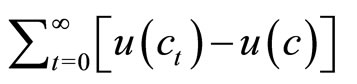 under a sequence of resource constraints:
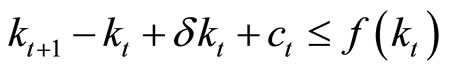 , to obtain the firstorder conditions:
 (16)
(16)
 (17)
(17)
We want to prove that the discrete-time system (16)- (17) is a discretization of the continuous-time system (14)- (15).
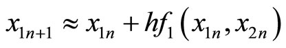
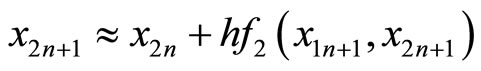
Proposition 7 The discrete-time Ramsey model comes from a first-order hybrid Euler discretization of the continuous-time model, that is a backward-looking discretization of the resource constraint (14) and a forwardlooking discretization of the Euler Equation (15), with a unit step.
Proof Under the backward-looking linear discretization of the continuous-time resource constraint (14):
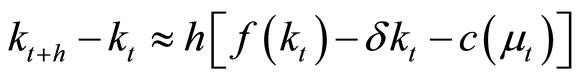 (18)
(18)
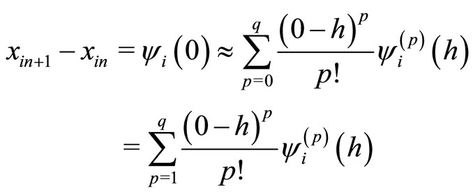
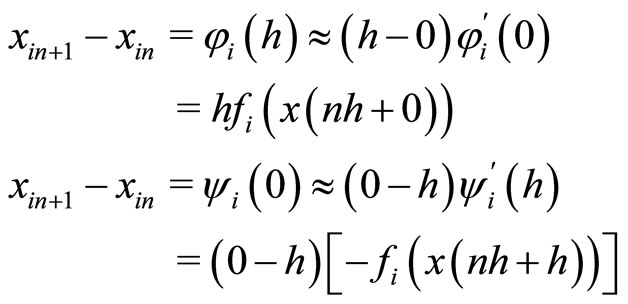
we recover exactly the discrete-time resource constraint (16) with a unit discretization step ( ). However, the intertemporal arbitrage requires a forward-looking discretization. Focus on (15) and apply (4):
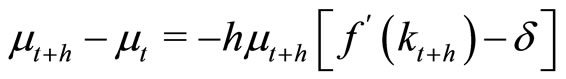
to obtain
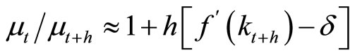 (19)
(19)
which gives exactly the discrete-time Euler Equation (17) under a unit discretization step .
.
The forward-looking discretization of (15) is more suitable to capture saving decisions. Indeed, the expected productivity affects the arbitrage between consumption today and consumption tomorrow.
Let us consider the steady state. For all the three dynamical systems (14)-(15), (16)-(17) and (18)-(19) the steady state is defined by: 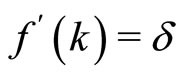 and
and 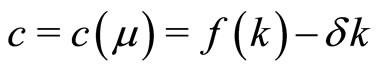 (assumptions on technology and preferences ensure its existence and uniqueness).
Focus now on the stability properties. The Jacobian matrix  of the continuous time system (14)-(15) is given by:
where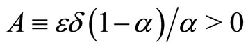 ,
, 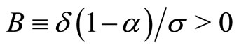 with
with
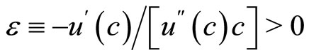 ,
, 
and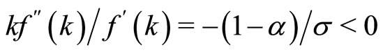 . The trace and the determinant in continuous time are
  and
and
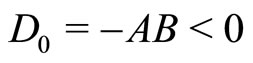 .
.
Notice that  implies the saddle-path stability property.
The hybrid Euler discretization (18)-(19) is consistent with the continuous-time case.
Proposition 8 The steady state of the discretized model is a saddle point (as in the continuous-time case) whatever the discretization step h.
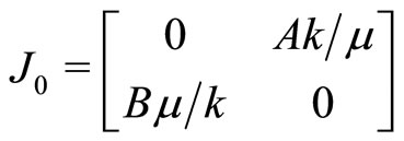
Proof The Jacobian matrix  of the hybrid Euler discretization (18)-(19) is:
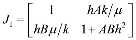
where A and B are defined above. The trace and determinant become 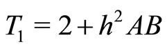 and
and . We obtain
  and we recover the saddle-path stability property, whatever the discretization step h. There is no room for bifurcations, as in the continuous-time case.
Therefore, the saddle-path stability is a robust property of the Ramsey model because it holds whatever the discretization step.
REFERENCES
- F. Ramsey, “A Mathematical Theory of Saving,” Economic Journal, Vol. 38, No. 152, 1928, pp. 543-559. doi:10.2307/2224098
- H. Krivine, A. Lesne and J. Treiner, “Discrete-Time and Continuous-Time Modelling: Some Bridges and Gaps,” Mathematical Structures in Computer Science, Vol. 17, No. 2, 2007, pp. 261-276. doi:10.1017/S0960129507005981
- P. A. Samuelson, “The Stability of Equilibrium: Comparative Statics and Dynamics,” Econometrica, Vol. 9, No. 2, 1941, pp. 97-120. doi:10.2307/1906872
- S. Bosi and L. Ragot, “Time, Bifurcations and Economic Applications,” CES Working Papers, 2009.28, University of Paris 1, 2009.