Journal of Mathematical Finance
Vol.2 No.2(2012), Article ID:19212,16 pages DOI:10.4236/jmf.2012.22017
Option Pricing Applications of Quadratic Volatility Models
1Department of Supply Chain Management, University of Manitoba, Winnipeg, Canada
2Department of Statistics, University of Manitoba, Winnipeg, Canada
Email: *appadoo@cc.umanitoba.ca
Received January 20, 2012; revised March 1, 2012; accepted March 16, 2012
Keywords: Garch Processes; RCA Models; Garch Models; Time varying volatility; Kurtosis
ABSTRACT
Recently there has been a surge of interest in higher order moment properties of time varying volatility models. Various GARCH-type models have been developed and successfully applied in empirical finance. Moment properties are important because the existence of moments permit verification of how well theoretical models match stylized facts such as fat tails in most financial data. In this paper, we consider various types of random coefficient autoregressive (RCA) models with quadratic generalized autoregressive conditional heteroscedasticity (GARCH) errors and study the moments, mean, variance and kurtosis. We also consider the Black-Scholes model with RCA GARCH volatility and show that these moments can be used to evaluate the call price for European options.
1. Introduction
It is well-known that many financial time series such as stock returns exhibit leptokurtosis and time-varying volatility [1]. The generalized autoregressive conditional heteroscedasticity (GARCH) and the random coefficient autoregressive (RCA) models have been extensively used to capture the time-varying behaviour of the volatility. Studies using GARCH models commonly assume that the time series is conditionally normally distributed; however, the kurtosis implied by the normal GARCH tends to be lower than the sample kurtosis observed in many time series Bollerslev [1]. Thavaneswaran et al. [2] use an ARMA representation to derive the kurtosis of various classes of GARCH models such as power GARCH, nonGaussian GARCH, non-stationary and random coefficient GARCH. Recently, Thavaneswaran et al. [3], Appadoo et al. [4] have extended the results to stationary RCA processes with GARCH errors and Paseka et al. [5] further extended the results to RCA processes with stochastic volatility (SV) errors.
Leptokurtosis is commonly observed in financial time series, as well as in currency and commodity markets. The opening and closure of the markets, time-of-the-day and day-of-the-week effects, weekends and vacation periods cause changes in the trading volume that translates into regular changes in price variability. Financial, currency, and commodity data also respond to new information entering into the market, which usually have large kurtosis. Recently, there has been growing interest in using volatility models [3,4]. Most of the studies use GARCH models with dummy variables in the volatility equation, and a few of them have been extended to a more flexible form such as the RCA GARCH. However, even though much research has been performed on volatility models applied to market data such as stock returns, more general specifications accounting for RCA with GARCH errors have been little explored. First we derive the kurtosis of a simple time series model with behaviour in the mean. Then we introduce various classes of RCA GARCH models and study the moments and discuss applications in option pricing. We extend the results for RCA GARCH volatility models to RCA quadratic GARCH models. The RCA GARCH model is appropriate for time series where significant autocorrelation exists. Option pricing with RCA model with quadratic GARCH errors is also discussed in some detail. The moments derived for the RCA GARCH volatility models provide more accurate estimates of market data behaviour and help investors, decision makers, and other market participants develop improved trading strategies. The rest of the paper is organized as follows. In rest of Section 1, we present results on standard GARCH models. These results are interesting for their own sake. In Section 2, we derive the higher order moments of some RCA models with GARCH errors, and in Section 3 we discuss some option pricing applications with RCA models with GARCH errors.
GARCH Models
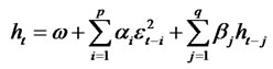
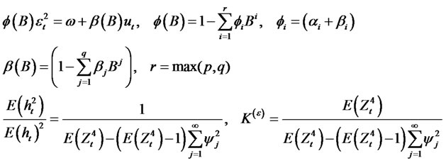
Consider the general class of GARCH (P,Q) model for the time series yt, where
 (1.1)
(1.1)
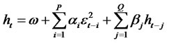 (1.2)
(1.2)
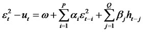
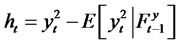
where Zt is a sequence of independent, normally distributed random variables with zero mean, unit variance. Let  be the martingale difference and let
  be the variance of
 , (2.12) and (1.2) could be written as:
 (1.3)
(1.3)
 (1.4)
(1.4)
 (1.5)
(1.5)
where
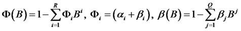
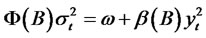
and R = max(P,Q).We shall make the following stationarity assumptions for  which has an ARMA(R,Q) representation.All the zeroes of the polynomial Φ(B) lie outside of the unit circle.
  where the
are obtained from the relation with
with
 . The assumption sensure that the
 are uncorrelated with zero mean and finite variance and that the
  process is weakly stationary. In this case, the autocorrelation function of
  will be exactly the same as that for astationary ARMA(R,Q) model. For any random variable ε with finite fourth moments, the kurtosis defined by
  and if the process {Zt}
is normal then the process {εt} defined by equations (1.3) and (1.4) is called a normal GARCH (p, q) process. The kurtosis ofthe GARCHprocess is denoted by  when it exists.
2. Random Coefficient Volatility Models
Consider the class of random coefficient autoregressive (RCA) models defined by allowing random additive perturbations of the autoregressive (AR) coefficients of ordinary AR models. That is, we assume that the process yt is given by,
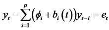 (2.1)
(2.1)
where the parameters θi, i = 2, ···, p, are assumed to be known,  and
and  are zero mean square integrable independent processes and the variances are denoted by
  and
and .
.  are independent of
  and
and  and may be thought of as incorporating structural changes. In order to motivate nonlinear forecasts for nonlinear models, we consider a class of estimating functions of the form
  [6], where
  and
and  is a function of
  and possibly the known parameters
  (i.e. We assume that the fitted model is available). If we restrict ourselves to a class of estimating functions of the above form then we can forecast the future value of
  based on the observed values
 as
as . That iswhether we have an AR(p) model or RCA(p) model we will get the same linear predictor of
 . However, for the RCA model under consideration, we have
 and
and .
.
Thus, the conditional variance is a nonlinear function and hence the RCA model may be viewed as a non-linear time series model. Nicholls and Quinn [7] studied linear as well as some nonlinear (proposed) forecast by fitting a nonlinear (RCA) model for the classical lynx cycle data. Using heuristic reasoning they proposed a nonlinear forecast and  theyshowed empirically that the forecast
  is a better predictor (having smalller forecast errors when compared with the actual observations) than the linear forecast for the lynx data. It is of interest to note that by defining
 , the optimal forecast for
  can be obtained as
 .
.
That is, the estimating function method can be used to obtain a nonlinear forecast for a nonlinear models by considering a class of elementary martingale estimating functions generated by nonlinear functions of the observations. Using a similar argument we could also obtain forecasts for various class of GARCH models, see Thavaneswaran and Heyde [6] for details. The main message is RCA models could be used to improve the forecasting performance of stochastic volatility models.
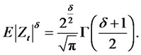
Lemma 2.1. When Zt is a standard normal random variable such that Zt ∼ N(0,1) then,
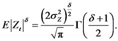
 Now if
  then
then
 As a general case for even powers we have
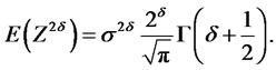
2.1. RCA Models
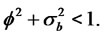
Random coefficient autoregressive time series were introduced by Nicholls and Quinn [10] and some of their properties have been studied recently by Thavaneswaran [3]. RCA models exhibiting long memory properties have been considered in Leipus and Sugailis [8]. A sequence of random variables {yt} is called an RCA (1) time series if it satisfies the equations
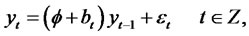
where Z denotes the set of integers and 1) 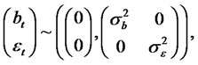
2) 
The sequences {bt} and {εt} respectively, are the errors in the model.
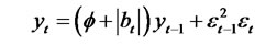
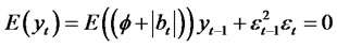
Theorem 2.1. Let {yt} be a modified RCA (1) time series with an absolute value random coefficient satisfying conditions (1) and (2). The modified RCA (1) model is given by
 (2.2)
(2.2)
 Then we have the following 1)
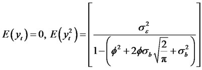
2) 
3) 
The autocovariance and the autocorrelation functions are given by
 and
and 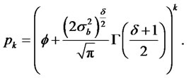
wang#title3_4:spProof:

Thus, we have
 (2.3)
(2.3)
and we have
 (2.4)
(2.4)
When , the kurtosis of the process yt converge to K(y) = 3. Thus, the autocorrelation function is given by

where we use the fact that ρ0 = 1.
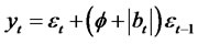
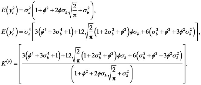
Theorem 2.2. Suppose yt is an Random Coefficient Moving average process model of the form
 (2.5)
(2.5)
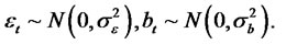
where bt is an uncorrelated Gaussian process with zero mean and with variance . εt is an uncorrelated Gaussian process with zero mean and with variance
 . Then, we have the following
Proof:
 (2.6)
(2.6)
and
We have
 (2.7)
(2.7)
and
Thus we have
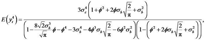
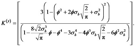
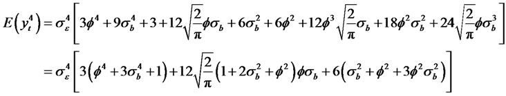
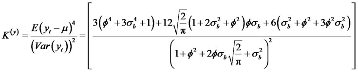
The kurtosis of the process is given by
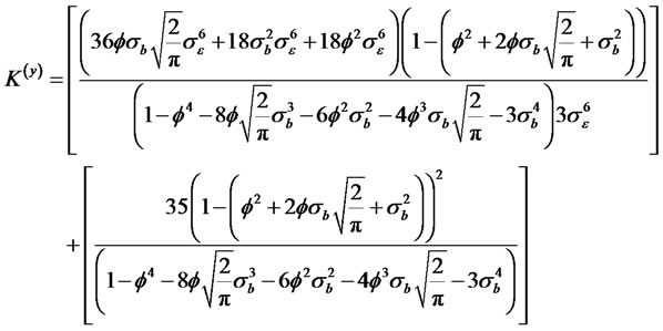 (2.8)
(2.8)
When , the kurtosis of the process yt converge to
 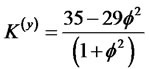 and when
 , and
, and  the kurtosis of the process yt turns out to be 35.
Theorem 2.3. Suppose yt is an Random Coefficient Moving average process model of the form
 (2.9)
(2.9)
where bt is an uncorrelated noise process with zero mean and with variance . εt is an uncorrelated noise process with zero mean and with variance
 . Then, we have the following relationships
and the autocorrelation functions are given by
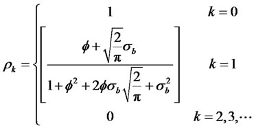 (2.10)
wang#title3_4:spProof:

Thus,
The autocorrelation function is given by

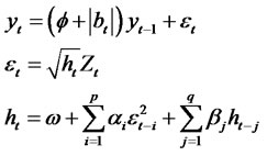
Theorem 2.4. Let {yt} be a Sign RCA-GARCH (1,1) time series satisfying conditions (i) and (ii) given by
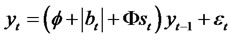 (2.11)
where
 (2.12)
 (2.13)
where Zt and bt are sequences of independent, identically distributed random variables with zeromean, variance given by  and
and  respectively,

ω, α1, β1 and Φ are real parameters, satisfying the following conditions, ω > 0, α1 ≥ 0, β1 ≥ 0. |Φx| ≤ ω. Note: , and in order to calculate the kurtosis, we observe that
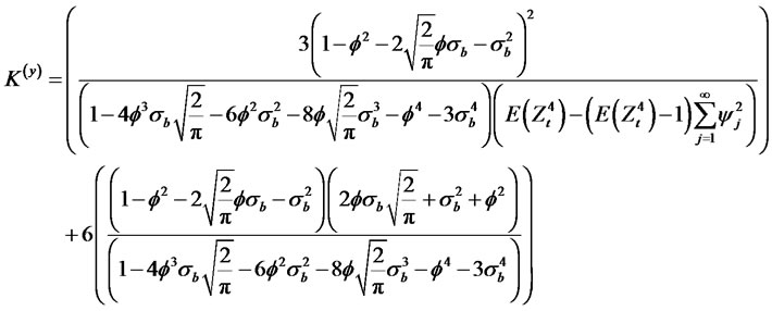
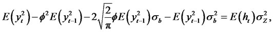
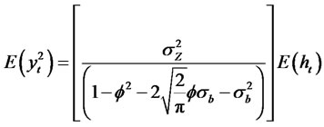
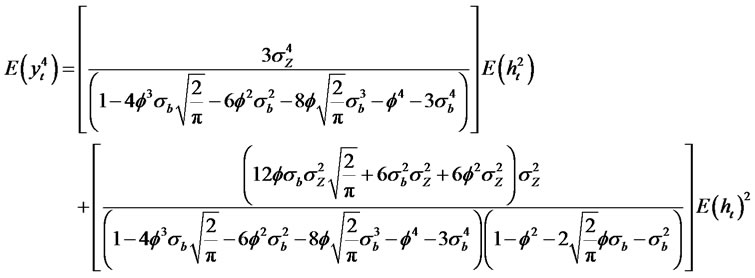
 . Then, we have the following moment properties
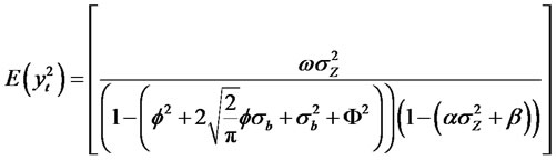
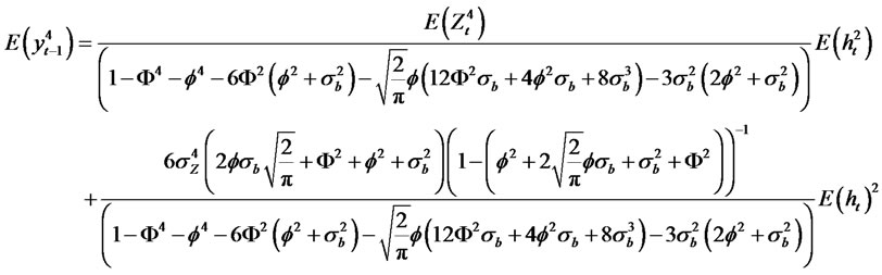
 (2.14)
Proof:

where

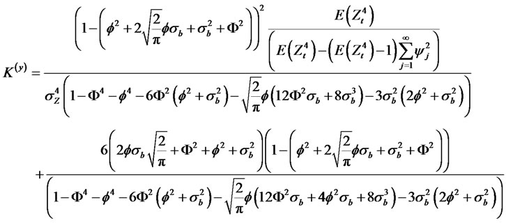
Using the facts that
Thus, we have the following expression for the Kurtosis of the process.
Special cases, for a Normal GARCH (1,1).
 (2.15)
Note, that when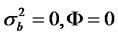 , and
, and  in (2.15), the kurtosis of the process converges to
 (2.16)
When  in (2.16),the kurtosis of the process converge to
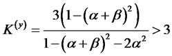
Theorem 2.5. Suppose yt is a modified RCA model with GARCH (p, q) innovations of the form
where bt is an uncorrelated noise process with zero mean and with variance  and Zt is an uncorrelatednoise process with zero mean and with variance
 . Then, we have the following relationship
 (2.17)
 (2.18)
 (2.19)
Proof: Let, 

Now we have
Thus,

and

 (2.20)

Using the fact that , we have
For convenience let  where,
The Kurtosis of the process is given by

Using the fact that  we have
 (2.21)
2.2. Quadratic GARCH Model
Besides having excess kurtosis market returns may display seriously skewed distributions. Linear GARCH models cannot cope with such skewness, and therefore we can expect forecast of linear GARCH model to be biased for skewed time series. To deal with this problem non-linear GARCH models are introduced, which take into account skewed distributions. The QGARCH model differs from model the classical GARCH model by
 (2.22)
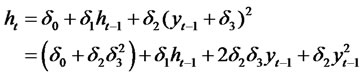 (2.23)
This model reduces to the GARCH (1,1) model when the shift parameters δ3 = 0. The QGARC Hmodel can improve upon the standard GARCH since they can cope with positive (or negative) skewness.
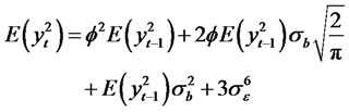
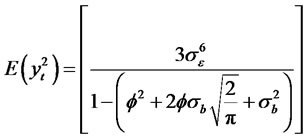
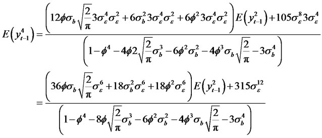
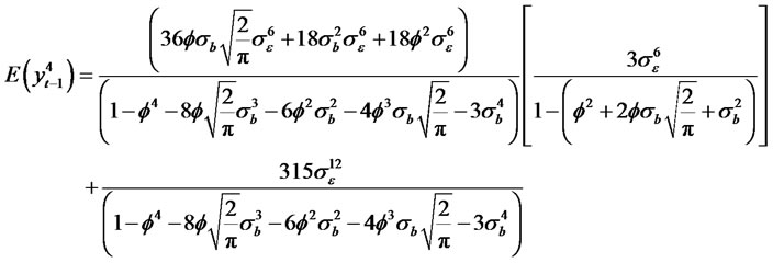
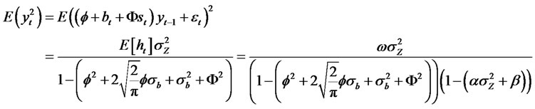
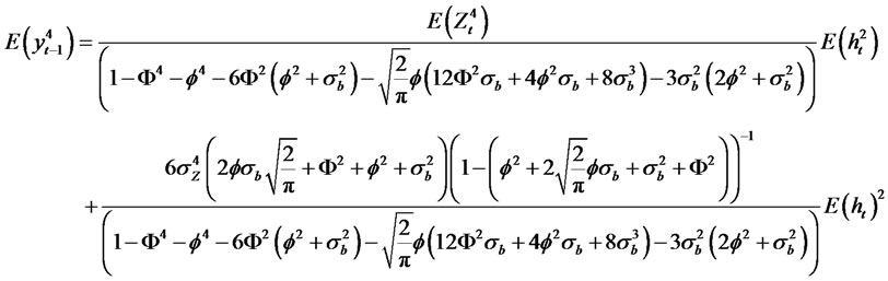
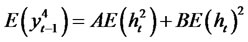
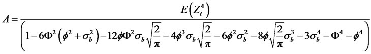
Theorem 2.6. Consider the general class of RCA QGARCH (1,1) Volatility Models for the time series yt, where
 (2.24)

(2.25)
where 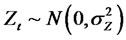 and
and . Then, we have the following moment properties

Proof: is easy and is omitted.
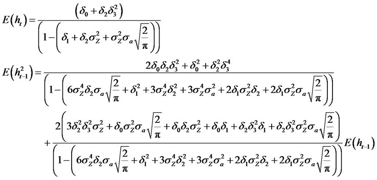
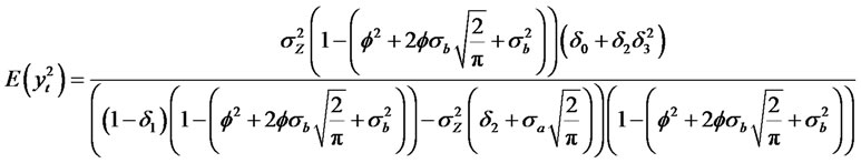
Theorem 2.7. Consider the special class of RCA QGARCH (1,1) Sign Volatility Models for the time series yt, where
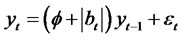 (2.26)
 (2.27)
 (2.28)
where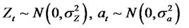 , at ∼N(0,σ2a) and
 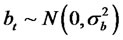 are sequences of independent, identicallydistributed random variables with zero mean, variance given by
  and
and  and
and  respectively, and

Note: , and in order to calculate the kurtosis, we observe that
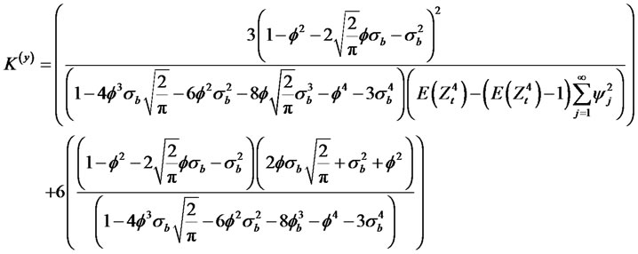
 . Then, we have the following moment properties
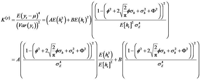
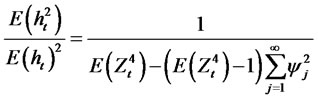
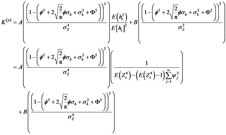
 (2.29)
 (2.30)
 (2.31)
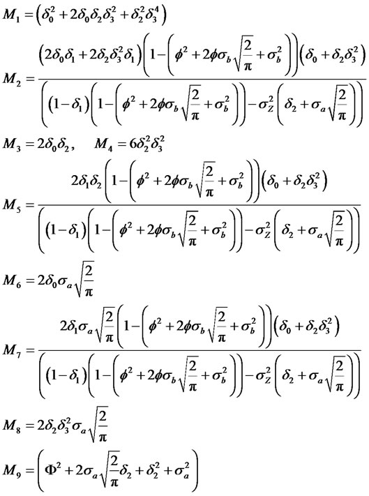
 (2.32)
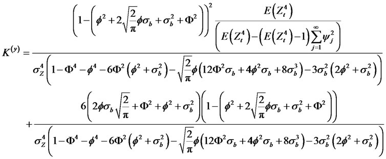
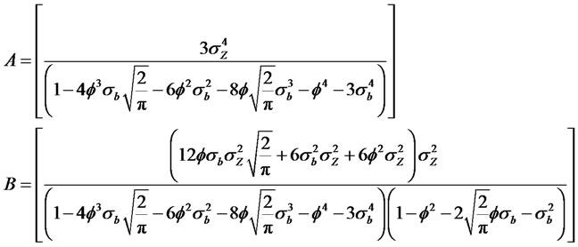
where
 (2.33)
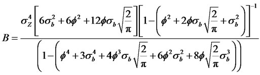 (2.34)
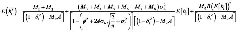 (2.35)
Proof: is easy and is omitted.
3. Option Pricing with Volatility
Option pricing based on the Black-Scholes model is widely used in the financial community. The BlackScholes formula is used for the pricing of European-style options. The model has traditionally assumed that the volatility of returns is constant. However, several studies have shown that assetre turns exhibit variances that change time [9,10,] and others derived closed form option pricing formulas for different models which are assumed to follow a GARCH volatility process. Most recently, Gong et al. [11] derive an expression for the call price as an expectation with respect to random GARCH volatility. The model is then evaluated in terms of the moments of the volatility process. Their results indicate that the suggested model outperforms the classic BlackScholes formula. Here we apply [11] and propose an option pricing model with RCA GARCH volatility as follows:
 (3.1)
(3.1)
 (3.2)
(3.2)
 (3.3)
(3.3)
where St is the price of the stock, r is the risk-free interest rate, {Wt} is a standard Brownianmotion, σt is the time-varying RCA GARCH volatility process, {Zt} is a sequence of i.i.d. randomvariables with zero mean and unit variance and Φ(B), and β(B) have been defined in (1.5). Theprice of a call option can be calculated using the option pricing formula given in [11]. The call priceis derived as a first conditional moment of a truncated lognormal distribution under the martingalemeasure, and it is based on estimates of the moments of the GARCH process. The call price basedon the Black-Scholes model with seasonal GARCH volatility is given by:
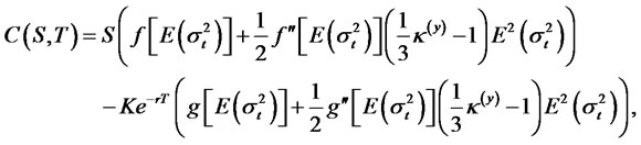 (3.4)
(3.4)
where f and g are twice differentiable functions, S is the initial value of St, K is the strike price, T is the expiry date, σt is a stationary process with finite fourth momentand .
.
Also,
and
are given by:

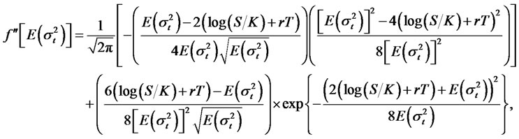
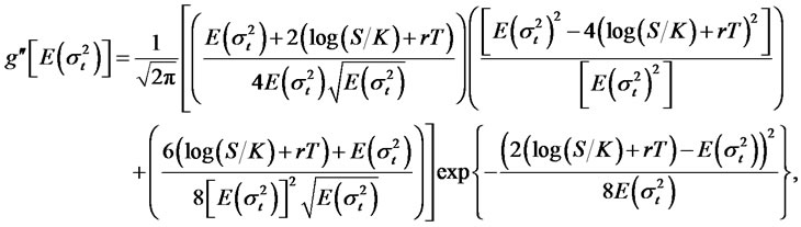
where N denotes the standard normal CDF, and under the option pricing model with RCA GARCH volatility,

4. Concluding Remarks
Financial time series exhibit excess kurtosis and in this paper, we propose various classes of RCAGARCH volatility models and derive the kurtosis in terms of model parameters. We consider time series models such as RCA with GARCH errors and quadratic GARCH errors. The models introduced here extend and complement the existing volatility models in the literature to RCA models with quadratic GARCH models by introducing more general structures. The results are primarily oriented to financial time series applications. Financial time series often meet the large data set demands of the volatility models studied here. Also, financial data dynamics and higher order moments are of interest to many market participants. Specifically, we consider the Black-Scholes model with RCA GARCH volatility and show that these moments can be used to evaluate the call price for European options.
REFERENCES
- T. Bollerslev, “Generalized Autoregressive Conditional Heteroscedasticity,” Journal of Econometrics, Vol. 31, No. 3, 1986, pp. 307-327. doi:10.1016/0304-4076(86)90063-1
- A. Thavaneswaran, S. S. Appadoo and M. Samanta, “Random Coefficient GARCH Models,” Mathematical and Computer Modelling, Vol. 41, No. 6-7, 2005, pp. 723- 733. doi:10.1016/j.mcm.2004.02.032
- A. Thavaneswaran, S. S. Appadoo and M. Ghahramani, “RCA Models with GARCH Errors,” Applied Mathematics Letters, Vol. 22, No. 1, 2009, pp. 110-114. doi:10.1016/j.aml.2008.02.015
- S. S. Appadoo, A. Thavaneswaran and S. Mandal, “RCA Models with Quadratic GARCH Innovations Distributions,” Applied Mathematics Letters, 2012, in Press.
- A. Paseka, S. Appadoo and A. Thavaneswaran, “Random Coefficient Autoregressive (RCA) Models with Nonlinear Stochastic Volatility Innovations,” Journal of Applied Statistical Science, Vol. 17, No. 3, 2010, pp. 331-349.
- A. Thavaneswaran and C. C. Heyde, “Prediction via Estimating Functions,” Journal of Statistical Planning and Inference, Vol. 77, No. 1, 1999, pp. 89-101. doi:10.1016/S0378-3758(98)00179-7
- D. Nicholls and B. Quinn, “Random Coefficient Autoregressive Models: An Introduction,” Lecture Notes in Statistics, Vol. 11, Springer, New York, 1982.
- R. Leipus and D. Surgallis, “Random Coefficient Autoregression,regime Switching and Lond Memory,” Advances in Applied Probability, Vol. 35, No. 3, 2003, pp. 737-754. doi:10.1239/aap/1059486826
- S. Heston and S. Nandi, “A Closed-Form GARCH Option Valuation Model,” The Review of Financial Studies, Vol. 13, No. 3, 2000, pp. 585-625. doi:10.1093/rfs/13.3.585
- R. Elliot, T. Siu and L. Chan, “Option Pricing for GARCH Models with Markov Switching,” International Journal of Theoretical and Applied Finance, Vol. 9, No. 6, 2006, pp. 825-841. doi:10.1142/S0219024906003846
- H. Gong, A. Thavaneswaran and J. Singh, “A BlackScholes Model with GARCH Volatility,” The Mathematical Scientist, Vol. 35, No. 1, 2010, pp. 37-42.
NOTES
*Corresponding author.