Open Journal of Marine Science
Vol.2 No.1(2012), Article ID:17063,8 pages DOI:10.4236/ojms.2012.21002
Management for the White Shrimp (Litopenaeus vannamei) from the Southeastern Gulf of California through Biomass Models Analysis
1Instituto Nacional de Pesca, Centro Regional de Investigación Pesquera, Mazatlán, México
2Posgraduate Program PCMyL, Universidad Nacional Autónoma de México, Mazatlán, México
Email: *juanchomvera@yahoo.com.mx
Received July 26, 2011; revised September 30, 2011; accepted October 8, 2011
Keywords: Litopenaeus vannamei; Biomass; Gulf of California
ABSTRACT
Samples taken during the closed fishing seasons from 1992 to 2010 were analyzed at sea. These data along with the landing records for the fishing periods from 1992-1993 to 2009-2010 were used to allow the situation of Litopenaeus vannamei from the coasts of Sinaloa and Nayarit to be analyzed by means of stochastic models and by a graphic approach for the surplus biomass. Using the catch from 1993-1994 as a reference point and comparing this to the 2008-2009 catch revealed a stock decrease of about 65%. By taking into account the percentage contribution to total shrimp landings, these changes showed a decrease from 76% to 12%. There were changes between 2000 and 2001 when the fleet grew by 50%. Considering a 3600 t maximum sustained yield (MSY) in the series 1992-2010, 50% of the reports are lower. It is necessary to recover the stock.
1. Introduction
We believe that updating of the present information and having a discussion about the Pacific white shrimp population, with the goal of revitalizing the protection and the future of the stock, is important. We may do this by generating a diverse heuristic approach on the present health of the population, its exploitation, and catch levels through biomass models and the associated graphic analysis.
From studies of the structure and population dynamics of the white shrimp in the continental area of the southern Gulf of California, the highest recruitment and greatest growth rates for penaidae shrimp was from June to July in the estuarine system Huizache and Caimanero at the mouth of the Gulf of California [1,2]. A decrease in the catch for the Pacific white shrimp is suggested by some work since 1956 for Central America, San Salvador, and Panama and is related to the growth in the fishing effort [3]. Is also recorded in the summer in estuarine system Huizache and Caimanero for the two Litopenaeus spp. [4]. From data for the mouth of Rio Baluarte, recorded that the highest abundance of postlarvae were from June to September for L. vannamei [5]. From data of L. vannamei of the Rio Presidio, also at the mouth of the California Gulf, determined that despite the spatial abundance variation, the postlarval shrimp abundance is higher in the shallow coastal waters than in the lagoons [6] (Table 1). From landing data observed that for Litopenaeus stylirostris and Litopenaeus vannamei the conspicuous mature gonadal period was in the spring and summer, although for Farfantepenaeus californiensis and F. brevirostris gonadal maturity is seen all during the year [7]. A discussion on dynamic biomass models for brown shrimp in the northern Gulf of California [8], showed fluctuations in total catch, from 3900 t during 1976-1977 to 1500 t during 1990-1991, increasing to almost 4000 t in 1997- 1998 (Table 1). These catch records show that they are less than the value of the maximum sustained yield (MSY) estimated with the process error estimator. Part of this variation in catch can be attributed to fluctuations in the fishing effort because the number of vessels decreased from almost 500 in 1979-1980 to 300 in 1993-1994. The decrease for Litopenaeus stylirostris was attributed primarily to overexploitation of the resource and viral disease [9-12]. The lack of the Colorado River freshwater discharge [13,14], even though L. stylirostris and Farfantepenaeus californiensis are euryhaline species that inhabit hypersaline habitats in large numbers of postlarvae and juveniles [15], has been discussed.
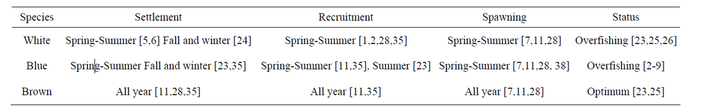
Table 1. Basic data of shrimp stocks in the Mexican Pacific.
Some workers believe the brown shrimp can respond immediately to the environment by changes in the first age of maturity, reproductive period, individual growth, and magnitude of recruitment [16]. The changes in distribution were evident when an El Niño affected the California current [17-21]. The El Niño caused a shift in the distribution of many taxa in the Pacific; including shrimp, fish, and mammals up to the northern range of the California current. In other models of the dynamic biomass population in Mexican waters, overfishing is assumed and there is a decline in shrimp landings [22,23].
In the lagoons of the Gulf of Tehuantepec, the abundance peaks of juvenile stages of the white shrimp occurred in December-January and March-May [24]. From data of the national fisheries bureau (INP) was made a recruit index and spawner abundances index from data of five closed seasons from May-June to August from 1993 to 1997 and four other fishing periods in the same years [25] (Table 1). By analyzing the annual variation for the brown shrimp (Farfantepenaeus californiensis) and white shrimp (Litopenaeus vannamei) in the Gulf of the Tehuantepec, the results indicated that the closed seasons protected almost 100% of the white shrimp recruits and 90% of the brown shrimp recruits. The brown shrimp fishery was in a good state because the abundances of the recruits and spawners were constant. The white shrimp fishery was in an overfished state because the number of the recruits and spawners were in decline [25]. An application used for surplus models is suggested in a lagoon in the Gulf of Tehuantepec for catch-per-unit effort (CPUE) from 1983 to 2006 [26]. The determination is by means of stationary enclosures and cast nets. The maximum shrimp production (806 t) was in 1987. Though the fishing effort remained constant since 1995, the shrimp landings are declining. The total shrimp production recorded for 2000 fell below 58% of the maximum sustainable yield (MSY) to 245 ton·y–1. The observed effort was 45% larger than the estimated effort at the MSY. The results reveal overexploitation, a declining abundance, and the risk of a collapse of the shrimp fishery in the area [26].
To assess the abundance of white shrimp stocks in the area of their heaviest density in the Pacific, the mouth of the Gulf of California (Figure 1), we used the reported catch and effort by the Comisión Nacional de Pesca y Acuacualtura [27] and evaluated this compared to the proportion of species reported by Instituto Nacional de Pesca [28]. We used, as an important reference and a framework for our study, the published literature on biomass data for Penaeus monodon in Australia [29,30].
In general, the analyzed catch and effort data for the white shrimp (Litopenaeus vannamei) fishery cover 18 years. We used data of some 3000 hauls made in the closed period from 1992 to 2010 and around 45 thousand landings in the fishing seasons from 1992-1993 to 2009- 2010. The average live-weight catch in the series analyzed is 1520 t. The largest catch is 5320 t of live weight in the 1993-1994 fishing season. The smallest catch was in 2000-2001 with about 430 t of live weight. In 2006- 2007 there is an increase to 2405 t live weight.
We used a dynamic biomass model in a stochastic version to analyze the catch-per-unit effort of the trawl fishery in the southeastern Gulf of California, Mexico, (Figure 1) where the major part of the Pacific fleet is concentrated. We assume that the CPUE is measured with an error, and there are other variability’s of the population that are produced by factors not included in the model. Moreover we recognize several sources of perturbation, such as changes in the size of the shrimp, in the recruitment, and in the environment. The environment and the
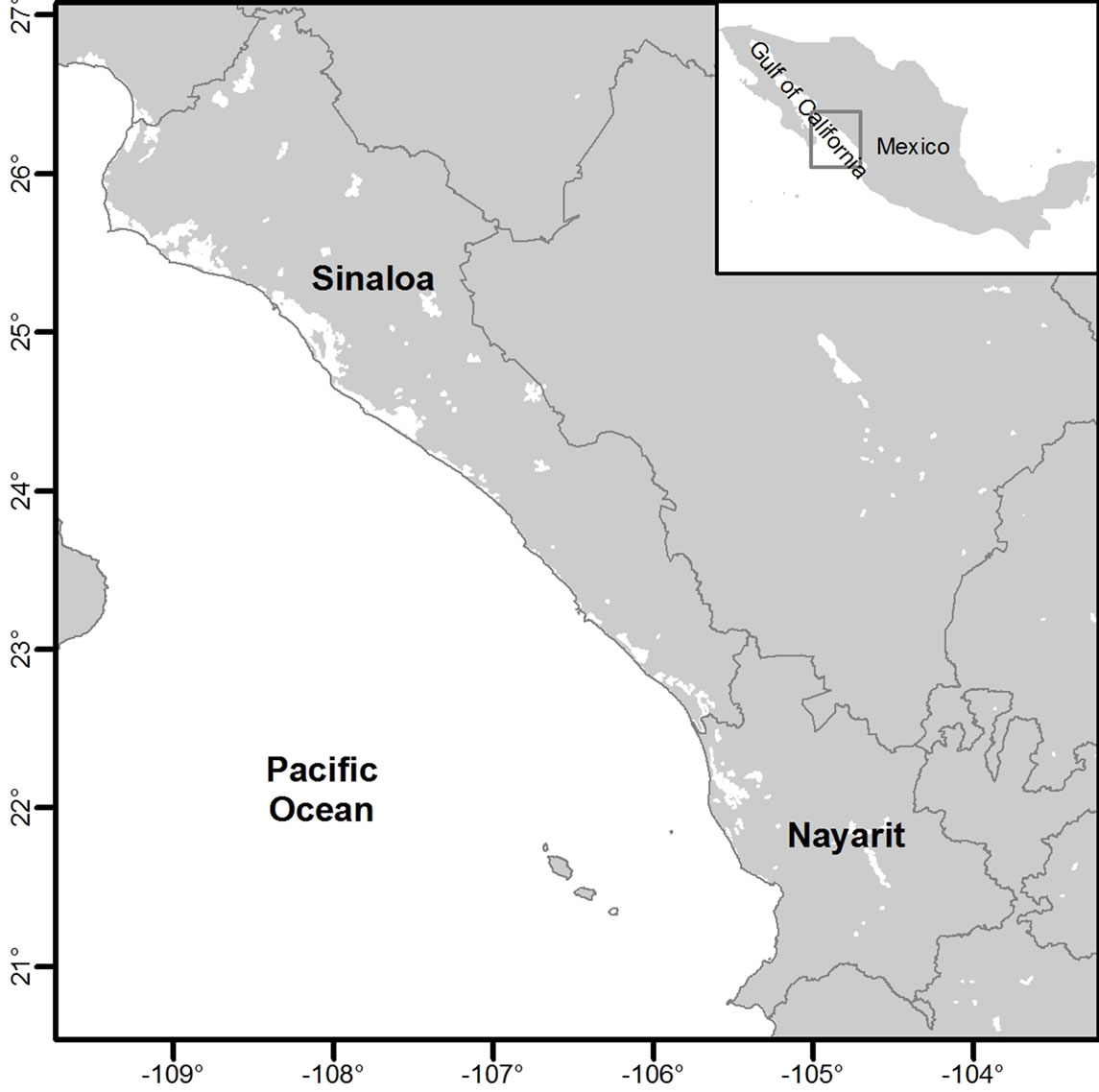
Figure 1. Study area in southeastern Gulf of California. Includes the continental shelf of Sinaloa and north of Nayarit, México.
fishing effects on the shrimp population are discussed as a hypothesis for the trends of the population and the CPUE.
2. Methods
To assess the abundance of white shrimp stocks we used the reported catch and effort by the CONAPESCA [27] and evaluated this compared to the proportion of species reported by the INAPESCA [28]. In general the work covers about 3000 hauls made in the closed periods from 1992 to 2010 by INAPESCA and around 45 thousand port landings in the fishing seasons from 1992-1993 to 2009-2010 by CONAPESCA. We defined the proportion of the contribution of the white shrimp to the total catch and the fleet number and estimated the CPUE in t per boat. The literature on biomass data published for Penaeus monodon in Australia [29,30] is well-suited as a reference. It is estimated to be a Schaefer Type [31] as amended by Pella-Tomlinson and discussed by Polachek et al. [32] in [33] such as
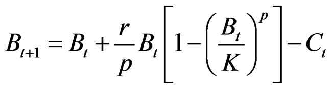
where Bt+1 is the predicted biomass at the time t + 1, Bt is the biomass at the time t, r is the growth rate, p is the function form parameter, K is carrying capacity, and Ct is the catch to time t.
The parameter model is estimated by maximizing the objective function of the type
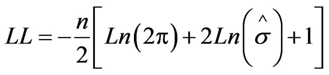
where LL is the log likelihood, n is the data number, and
 , where It is the CPUE observed and
  is the CPUE expected or qtBt, where q is the expected catchability in the time t and B is the predicted biomass in time t.
The confidence intervals are calculated at 95%, and the model parameters are made by the bootstrapping of the CPUE [33,34]. In each run of a thousand optimizations, it resets the surplus production model by replacing the values of the CPUE by that of the bootstrap. It is nonlinear, using the quadratic estimate, derived from a progressive and Newton algorithm 1000 times for each run.
The projections are made using the calculated model and the value of the initial capture or the observed CPUE and time (18 years), and the value of the observed effort, in this case 772 ± 100 ships, which are recorded in Nayarit and Sinaloa.
The catchability or q in the model was produced by q' = Ln(CPUE/Bt + 1), where CPUE is the value for the catch in the fishing period and Bt + 1 is biomass in time t + 1 for the Schaefer model vs time (18 fishing periods). In general, the case analyzed is assumed to be increasing by a constant amount each fishing period. The qt value for each year is produced from the linear equation qt = q0 + t * qadd, where qt is the catchability in year t, q0 is the start catchability, qadd is a constant amount by q increaseing each fishing period. The estimation of two parameters involves finding the gradient, qadd and intercept q1 of the linear regression between qt and time [33]. The model may be used for a decreasing case.
The model must be taken heuristically. The CPUE is calculated for the harvest season. We evaluated the history of the fishery between 1992 and 2000 and from 2001 to 2010. We evaluated and presented the model, in general, for the CPUE and effort and for the time. We calculated the surplus production model and presented this for the catch seasons. We calculated the likelihood adjustment of the parameters r, K, p, and the initial biomass Bo, which is the capture at the beginning of the series. We calculated the confidence intervals. The MSY is assessed, which assesses the projections using the model and the initial setting q. We also believe that the model behavior includes the descending data.
3. Results
The study area was in the southern Gulf of California and includes an area of 1500 km2 with depths from 8 m to 76 m or ~5 to ~42 fathoms (Figure 1).
These marine data are from the fishery institute in Mexico produced for the white shrimp from 1992 to 2010. The average live-weight catch in the series analyzed is 1520 tonnes (t) with a standard deviation of 1205 tonnes (t). The largest catch is 5320 t live weight in the 1993- 1994 fishing season (Figure 2). The smallest catches were in 2000-2001 and 2001-2002 with about 430 t and 460 t live weight. In 2003-2004 there is an increase of about 2380 t, and in 2006-2007 again an increase to 2400 t live weight.
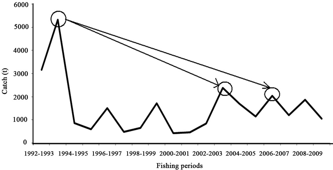
Figure 2. White shrimp catch from series of reported catch and proportion by INAPESCA data, for the southeastern Gulf of California. The maximum is 5320 tonnes (Modified from [38]).
These marine data are from penaoeidea assemblages, with the white shrimp populations off the coast of Sinaloa and Nayarit contributing about 17% (arithmetic average) of the catch of the fleet. The highest proportions were recorded in 1992 and 1993 with about 50% and 76%, and the lowest in 2000-2002 at about 5%. The most recent data for 2009-2010 is nearly 12% [23,35,36,28]. In 1993-1994, the white shrimp is first and from 1994 to 2010 was third in production, after the blue and the brown shrimp. The evaluation of the rebound in 2003-2004 compared to the catch of 1993-1994 is a loss of 56% (Figure 2). If we evaluate the rebound in 2006-2007 and 2008-2009 compared to 1993-1994, these are losses of between 62% and 65%.
Looking at the trend of the CPUE graphically (Figure 3), it is possible to make up two different histories (Figure 3(a)) in relation to changes in the effort, which is represented in the qualitative circles; one that the effort is nearly 550 boats ± 100 boats and other is 775 boats ± 100 boats. In part (b) of the figure, the period is from 1992 to 1999, and the extreme data is for the 1992-1993 and 1993-1994 fishing periods, with the ordinate scale amounting to 10 t. In part (c) for the period from 2000-2001 to 2008-2009, the scales change from (b) to (c) from 10 t to 5 t per boat. The extreme values in (c) are for 2003- 2004.
At the next step we adjusted the dynamic biomass model and the confidence interval generation, which is shown in Figure 4 (part (a)). The model and data have skewed the changes after 1993-1994. After 1994-1995, the CPUE remained at lower values, with the more critical in 2000-2001 and 2001-2002, shown by arrows. In (b)-(e) the precision is fitted for the r, k, Bo, and p parameters. The r value is 0.34, near to the values of Penaeus monodon that is a framework and considered the values for the logistic theory. The K values related to biomass in the context of carrying capacity is near 43,000 t, which is not an artifact if we take the area as 1500 km2 and assume values < 3 t per km2 per year. Bo is a value at the start of the series and increases to about 3375. The p value is 0.001, far from 1, a value similar to the classical Schaffer model and assuming tonnes (t) skewed to the right, a classic form for the function. The value for log likelihood was nearly –3.64 and the exponential was 0.02. If the null hypothesis is referred to than the dispersion of the CPUE calculated and observed may be explained by a log normal distribution.
When the scenario of the maximum sustained yield (MSY) and the effort to attain this maximum is considered, the MSY values were taken with the necessary care only heuristically. The MSY is nearly 3675 t live weight (Figure 5(a)) or 2450 t of tails. The effort for the MSY amounts to 145 boats (Figure 5(b)) with a maximum of 250 boats. In Figure 5 part (c), we added a relative test to predict under the MSY more than 83%, shown in the histogram and under the accumulated proportion curve. In Figure 5 part (d) we added another relative test of effort that predicted under the MSY more than 63%, shown in the histogram and under the accumulated proportion curve. In considering the catch series deduced from the proportion by the National Fishery Bureau and the official report of the catch by CONAPESCA, the catch is below the MSY in >90% of the data. If the effort report is minus 100 boats, then the effort is at least four times for this species and at least double if considering the maximum in the figure. The status of the stocks is deteriorating, given the current efforts and under the precautionary approach.
In the Figure 5 we represented the output for bootstrap for the MSY (part (a)) and the effort (part (b)) from the general model. In part (c) is the output for the predicted catch that was around the MSY, with at least 85% accounted for from the general model. In part d are the output effort values, which were near to the reported values and explained at least 65%. That is the framework for the model as a heuristic approach The simulation through bootstrap for the catchability or q = Ln(CPUE/Bt + 1) and the value produced for the regression for q compared to the time-series from 1 to 18 fishing periods that produced q'. We take the starting gradient and the intercept with the values of 0.95 and 0.00237. The r2 value for q was nearly 0.41 in the starting values. The bootstrap produces r2 values from 0.41 to >0.51. The r2 values for q0* qinic (when q0 and qinic were the gradient and the intercept for q respect the time),
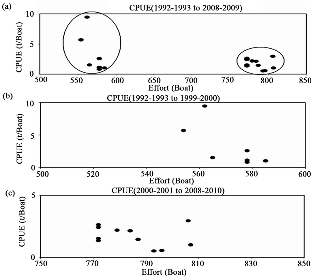
Figure 3. White shrimp catch per unit effort from a series of reported catch and effort in boats, for the southeastern Gulf of California. In part (a) the period from 1992-1993 to 2008- 2009. In (b) the period from 1992-2993 to 1999-2000 (Left circle in (a)). In (c) from 2000-2001 to 2008-2009 (the right circle in (a)). The scales change from (b) to (c) from 10 t to 5 t per boat.
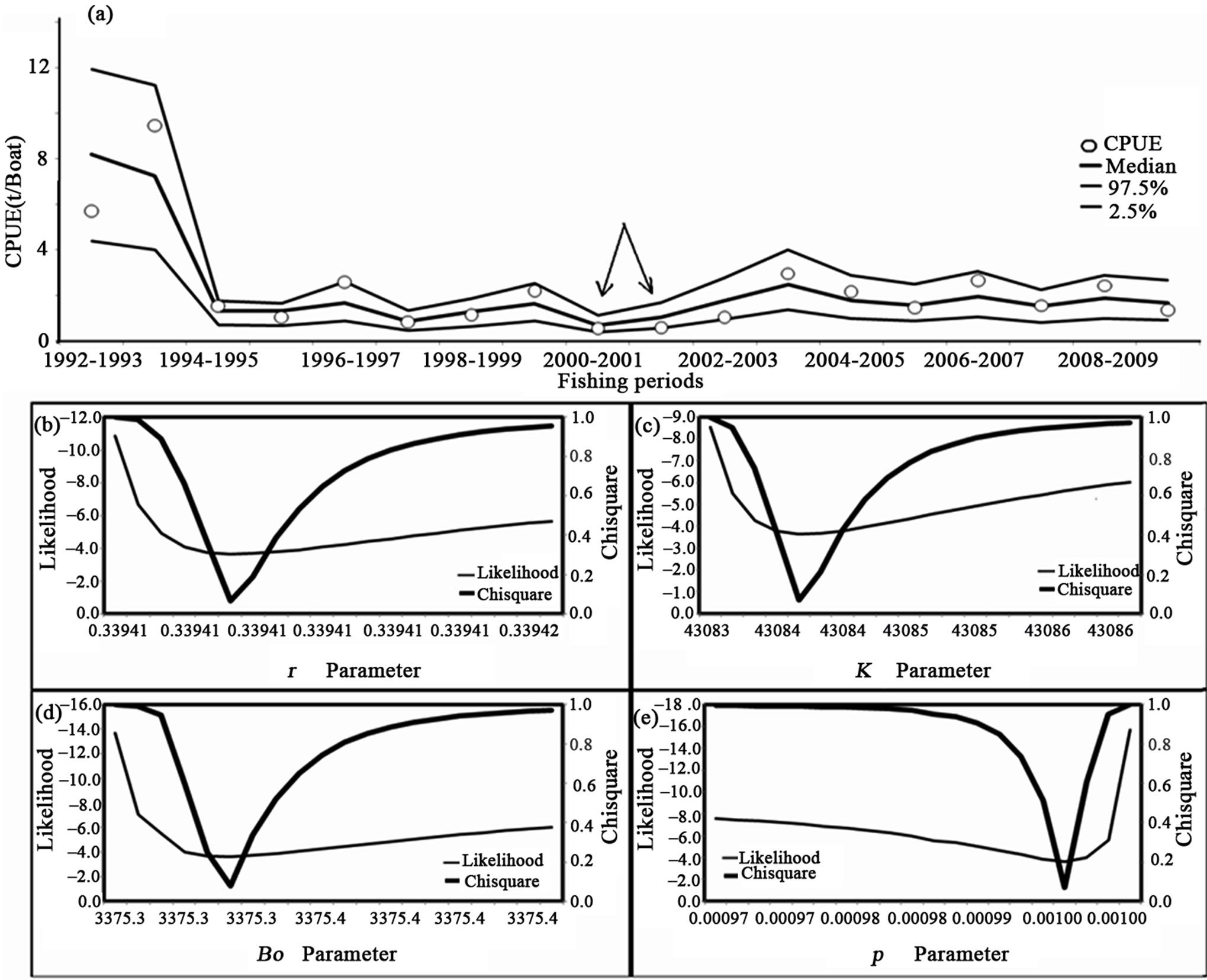
Figure 4. White shrimp dynamic model compared to the catch per unit effort from series of reported catch and effort in boats, for the southeastern Gulf of California. In the model and the confidence interval at 95% produced by bootstrap. In (b), (c), and (d) the precision fitted for the r, k, Bo, and p parameter. The fitting is only considered under bootstrap.
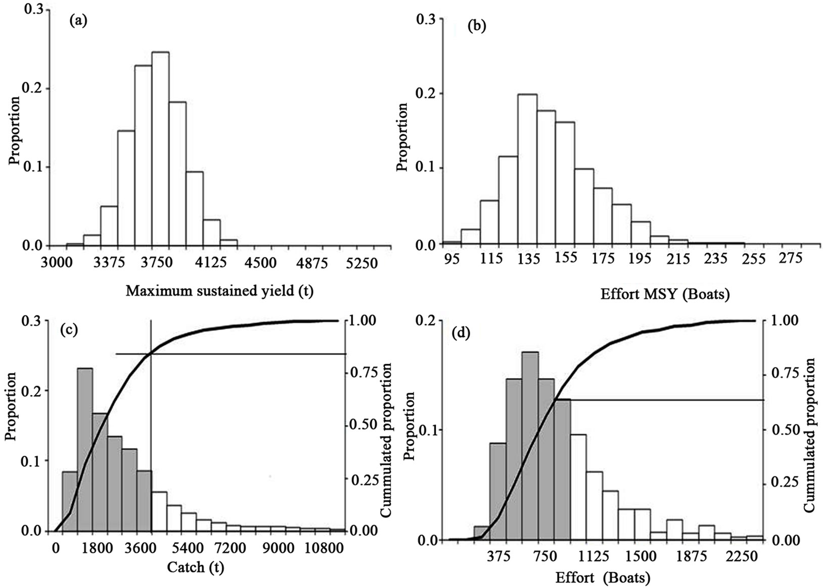
Figure 5. The maximum sustained yield (a) and effort (b) evaluation for the white shrimp. In figures a relative test for predicted catch (c) and effort (d) using the bootstrap routines. The dark area and accumulated proportion were considered the fit for the observed data and simulation. The catch and effort were that reported from 1992 to 2010.
by default were >0.9, with the q not increasing during the years, but decreasing. In Figure 6, the catchability bootstrap evaluation for the biomass dynamic model for the white shrimp is shown. In part (a) are the q values per fishing period. The variation is highest, such as is seen in the interval values with three and two orders of magnitude or zero values. In (b) are the q' values showing a constant interval that is about 0.003. In (c) are the median and confidence intervals for qt compared to the starting q and q', with the values not increasing. The line along part (c) is only qualitative.
4. Discussion
The diverse problems that are important for the implementation of the model are first the heuristic approach to understand the health status [37] of the white shrimp population. At the next step, we accept that the reported data have an observation error, such as the fleet size, that can fluctuate about one hundred vessels, because of mechanical or technical problems. The fleet has two components; one landing at Mazatlán and other fleet landing in the north at Topolobampo. The fleet size in 2001 to 2011 has 560 vessels landing at Mazatlán and nearly 100 at Topolobampo. Other problems are related to the underreported catch.
For the problems with the fleet size and the reported catch, we believe these changes may be included in the simulation made for the development models. For example, following the rules of random allocation of the observed CPUE compared to the observed catch, which can produce changes in the size of the effort, and which is measured in the number of boats and produces a scenario at least to explain >55% of the variance or dispersion. The model could explain a higher variance. The fit may continued in successive steps, including a higher dispersion. But the result may be considered a good approach and explain at least 55% of the results.
To explain the dispersion, we assumed that the status of Litopenaeus vannamei populations off the coast of Sinaloa and Nayarit may be deteriorating. From the catch in 1993-1994, the stock may be declining if compared with that of 2008-2009, with a decrease of 65%. The percentage contribution to the total catch of penaeids changes from 76% to 12%. The change happens between 2000 and 2001 when the fleet grows by 50%. If the MSY of 3600 t is compared to the catches from 1992 to 2010, 50% of the reports are under this MSY value and may mean overfishing. The r of the population related to mortality is >0.16. Then the decline in the stock has a continuous risk.
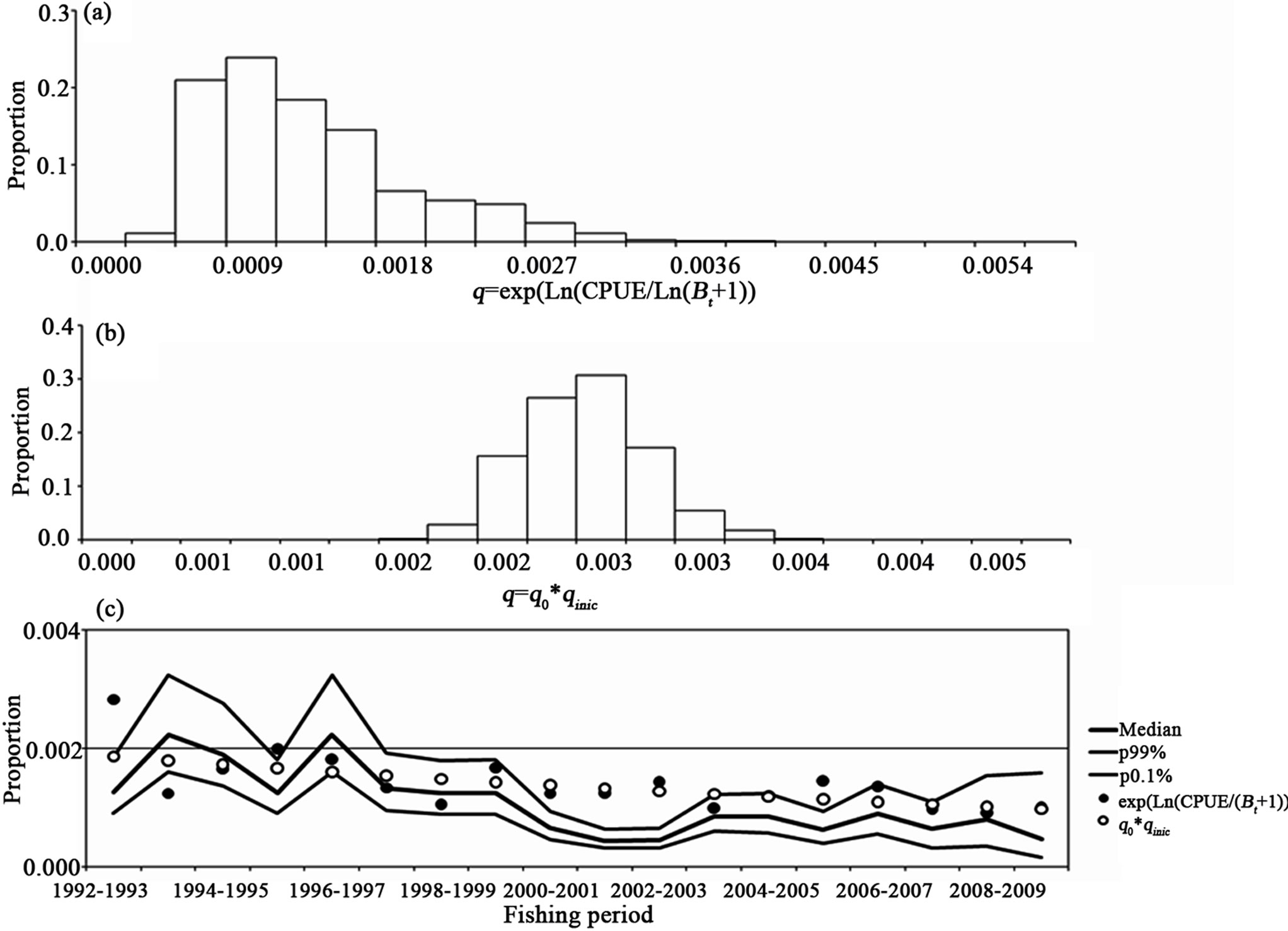
Figure 6. The catchability bootstrap evaluation for the white shrimp. In (a) is the q values per fishing period. In (b) are the q´ values considering a constant interval amount. In (c) the median and confidence intervals for qt are compared to the starting q and q'.
The implications can be that the population of white shrimp in the mouth of the Gulf of California is declining. Also, there may be the decline of breeding stocks and thus low success rates of larval and postlarval survival, with low rates of settlement in protected waters and shallow waters like those of depths of 0 to 5 fathoms. Moreover a byproduct is the decline in the CPUE. A decline in the CPUE is related to lower profit, lower capital, and lower wealth of the region, and so a lower welfare of the fishermen. There may be increased levels of conflict and a risk in the future of local shrimp populations. The stock recovery is important for the environment in the region and the management tools such as the closed season, a sustained fleet size, quotas, the protection of shallow marine waters, and no fishing areas are possible to be used.
5. Acknowledgements
To national fisheries bureau for data use and the support of technical staff of the shrimp program of INAPESCA. Thanks to Dr. Ellis Glazier for editing this English-language text.
REFERENCES
- R. R. C. Edwards, “The Fishery and Fisheries Biology of the Penaeid Shrimp on the Pacific Coast of Mexico,” Oceanography Marine Biology Annual Review, Vol. 16, 1978, pp. 145-180.
- A. Menz and A. B. Bowers, “Bionomics of Penaeus Vannamei Boone and P. stylirostris Stimpson in a Lagoon on the Mexican Pacific Coast,” Estuarine, Coastal and Marine Science, Vol. 10, No. 6, 1980, pp. 685-697. doi:10.1016/S0302-3524(80)80096-X
- L. D’Croz, F. Chérigo and N. Esquivel. “Observaciones sobre la Biología y Pesca del Camarón Blanco (Penaeus spp.) en el Pacifico de Panamá,” Anales del Instituto de Ciencias del Mar y Limnología Universidad Nacional Autónoma de México, Vol. 12, No. 1, 1978, pp. 144-153.
- C. R. Poli and J. A. Calderón-Pérez, “Efecto de los Cambios Hidrológicos en la boca del río Baluarte sobre la Inmigración de Postlarvas de Penaeus vannamei Boone y P. stylirostris Stimpson al Sistema Huizachie-Caimanero, Sin. México,” Anales del Instituto de Ciencias del Mar y Limnología Universidad Nacional Autónoma de México, Vol. 14, No. 1, 1985, pp. 29-44.
- C. R. Poli and J. A. Calderón-Pérez, “A Physical Approach to the Postlarval Penaeus Immigration Mechanism in a Mexican Coastal Lagoon (Crustacea: Decapoda: Penaeidae),” Anales del Instituto de Ciencias del Mar y Limnología Universidad Nacional Autónoma de México, Vol. 14, No. 1, 1987, pp. 147-156.
- R. Solis-Ibarra, J. A. Calderón-Pérez and S. RendónRodríguez, “Abundancia de Postlarvas del Camarón Blanco Penaeus vannamei (Decapoda: Penaeidae) en el litoral del Sur de Sinaloa, México, 1984-85,” Revista Biología Tropical, Vol. 41, No. 3, 1993, pp. 573-578.
- H. Garduño-Argueta and J. A. Calderón-Pérez, “Abundancia y Maduración Sexual de Hembras de Camarón (Penaeus spp.) en la Costa sur de Sinaloa, México,” Ciencias Marinas, Vol. 1, 1994, pp. 27-34.
- E. Morales-Bojórquez, J. López-Martínez and S. Hernández-Vázquez, “Dynamic Catch Effort Model for Brown Shrimp Farfantepenaeus Californiensis (HOLMES) from the Gulf of California, Mexico,” Ciencias Marinas, Vol. 27, No. 1, 2001, pp. 105-124.
- J. A. Rosas-Cota, V. M. García-Tirado and J. R. Gonzá- lez-Camacho, “Análisis de la Pesquería de Camarón en Altamar en San Felipe B.C. Durante la Temporada de Pesca 1995-1996,” Boletín CRIP, Inp-Semarnap, Vol. 2, 1996, pp. 23-30.
- A. Hernan, “Morphologic and Genetic Characterization of Wild Populations of Shrimp of the Genus Penaeus within the Gulf of California, Mexico: New Social, Political and Management Dilemmas for the Mexican Shrimp Fishery,” University of Arizona, Tucson, 1997.
- Instituto Nacional de la Pesca, “Evaluación de la Migración y Reclutamiento de las Poblaciones de Camarón en Aguas Protegidas y en el Frente Costero de Sinaloa y Sonora,” Informe Técnico, CRIP, Guaymas, 2002.
- A. S. Medina and L. A. Soto, “Assessment of the Fishing Effort Level in the Shrimp Fisheries of the Central and Southern Gulf of California,” World Fish Quarterly, Vol. 26, No. 4, 2003, pp. 16-20.
- M. S. Galindo-Bect, E. P. Glenn, H. M. Page, K. Fitzimmons, L. A. Galindo-Bect, J. M. Hernandez-Ayón, R. L. Petty, J. García-Hernández and D. Moore, “Penaeid Shrimp Landing in the Upper Gulf of California in Relation to Colorado River Freshwater Discharge,” Fish Bull, Vol. 98, 2000, pp. 222-225.
- E. A. Aragón-Noriega and E. Alcántara-Razo, “Influence of Sea Surface Temperature on Reproductive Period and Size at Maturity of Brown Shrimp (Farfantepenaeus Californiensis) in the Gulf of California,” Marine Biology, Vol. 146, No. 2, 2005, pp. 373-379. doi:10.1007/s00227-004-1442-3
- R. C. Brusca, “Common Intertidal Invertebrates of the Gulf of California,” University of Arizona Press, Tucson, 1980.
- J. López-Martínez, F. Arreguín-Sánchez, S. HernándezVázquez, A. García and W. Valenzuela, “Interannual Variation of Growth of the Brown Shrimp Farfantepenaeus californiensis and Its Relation to Temperature,” Fisheries Research, Vol. 61, No. 1-3, 2003, pp. 95-105. doi:10.1016/S0165-7836(02)00239-4
- P. C. Fiedler, “Some Effects of El Niño 1983 on the Northern Anchovy,” California Cooperative Oceanic Fisheries Investigations Reports, Vol. 25, 1984, pp. 53-58.
- T. L. Hayward, “Preliminary Observations of the 1991- 1992 El Niño in the California Current,” California Cooperative Oceanic Fisheries Investigations Reports, Vol. 4, 1993, pp. 21-29.
- T. L. Hayward, “El niño 1997-98 in the Coastal Waters of Southern California: A Timeline of Events,” California Cooperative Oceanic Fisheries Investigations Reports, Vol. 41, 2000, pp. 98-116.
- V. J. Madrid and P. Sánchez, “Patterns in Marine Fish Communities as Shown by Artisanal Fisheries Data on the Shelf off Nexpa River, Michoacán, México,” Fisheries Research, Vol. 33, No. 1-3, 1997, pp. 149-158.
- R. N. Lea and R. H. Rosenblatt, “Observations on Fishes Associated with the 1997-98 EI Niño off California,” California Cooperative Oceanic Fisheries Investigations Reports, Vol. 41, 2000, pp. 117-129.
- E. Morales-Bojórquez, V. M. Gómez-Muñoz, R. FélixUraga and R. M. Alvarado-Castillo, “Relationship between the Temperature and Density Independent Mortality of the Pacific Sardine Sadinops Sagas from Western Coast of Baja California Peninsula, Mexico,” Science Marine, Vol. 67, No. 1, 2003, pp. 25-32.
- Instituto Nacional de la Pesca, “Sustentabilidad y pesca Responsable en México. Evaluación y Manejo,” INP, SAGARPA, México, 2001, p. 1111.
- G. Rivera-Velázquez, L. A. Soto, I. H. Salgado-Ugarte and E. J. Naranjo, “Growth, Mortality and Migratory Pattern of White Shrimp (Litopenaeus vannamei, Crustacea, Penaeidae) in the Carretas-Pereyra Coastal Lagoon System, Mexico,” Revista Biología Tropical, Vol. 56, No. 2, 2008, pp. 523-533.
- P. Cervantes-Hernández, M. I. Gallardo-Berumen, S. Ramos-Cruz, M. A. Gómez-Ponce and A. Gracia-Gasca, “Analysis of the Closed Seasons in the Marine Shrimp Exploitation of the Gulf of Tehuantepec, Mexico,” Revista de Biología Marina y Oceanografía, Vol. 43, No. 2, 2008, pp. 285-294.
- G. Rivera-Velázquez, L. A. Soto, I. H. Salgado-Ugarte and E. J. Naranjo, “Assessment of an Artisanal Shrimp Fishery of Litopenaeus Vannamei in a Lagoon-Estuarine System Based on the Concept of Maximum Sustainable Yield,” Revista de Biología Marina y Oceanografía, Vol. 44, No. 3, 2009, pp. 635-646.
- Comisión Nacional de Acuacultura y Pesca, “Anuario Estadístico de Acuacultura y Pesca,” CONAPESCA, SAGARPA, México, 2008.
- Instituto Nacional de Pesca, “Resultados del Análisis de las Poblaciones de Camarón del Litoral del Pacífico para Implementar la Veda durante 2009,” Informe de Investigación, INAPESCA, SAGRAPA, 2009.
- R. Hilborn and C. J. Walters, “Quantitative Fisheries Stock Assessment: Choice, Dynamics and Uncertainty,” Chapham & Hall, New York, 1992.
- M. Haddon, “Modelling and Quantitative Methods in Fisheries,” Chapman and Hall/CRC, 2011.
- M. B. Schaefer, “Some Aspects of the Dynamics of Populations Important to the Management of Commercial Marine Fisheries,” Bulletin International American Tropical Tuna Community, Vol. 1, 1954, pp. 25-56.
- T. Polachek, R. Hilborn and A. Punt, “Fitting Surplus Productions Models: Comparing Methods and Measuring Uncertainty,” Canadian Journal of Fisheries and Aquatic Sciences, Vol. 50, 1993, pp. 2597-2607. doi:10.1139/f93-284
- M. Haddon, “Modelling and Quantitative Methods in Fisheries,” Chapman and Hall/CRC, 2001.
- M. H. Prager, “A Suite of Extensions to a Nonequilibrium Surplus-Production Model,” Fishery Bulletin, Vol. 92, 1994, pp. 374-389.
- Instituto Nacional de la Pesca, “Análisis de las Poblaciones Explotadas de Camarón Durante la Veda del 2004 en el Litoral del Pacífico Mexicano,” Informe de Investigación, INP, SAGARPA, 2004.
- Instituto Nacional de la Pesca, “Resultados de los Muestreos de las Poblaciones de Camarón, durante la Veda del 2007 en el Litoral del Pacífico,” DGIPPN, INP, SAGARPA, 2007.
- T. A. Branch, O. P. Jensen, D. Ricard, Y. Ye and R. Hilborn, “Contrasting Global Trends in Marine Fishery Status, Obtained from Catches and from Stock Assessments,” Conservation Biology, Vol. 25, No. 4, 2011, pp. 777-786. doi:10.1111/j.1523-1739.2011.01687.x
- INAPESCA, “Dictamen de cuota de camarón azul. Manejo Compartido por Cuotas para la Pesquería de Camarón azul Litopenaeus stylirostris: modelo Basado en Estructura de Tallas, Temporada 2010/2011 para las Aguas Protegidas, Ribera y alta mar de las Costas de Sinaloa,” INAPESCA, México, 2010.
NOTES
*Corresponding author.