Open Journal of Statistics
Vol.1 No.2(2011), Article ID:6520,12 pages DOI:10.4236/ojs.2011.12006
Parameter Estimations for Generalized Rayleigh Distribution under Progressively Type-I Interval Censored Data
1Department of Mathematical Sciences, University of South Dakota, Vermillion, USA
2School of Nursing, University of Rochester Medical Center, Rochester, USA
3Department of Statistics, Tamkang University, Taipei, China
E-mail: Yuhlong.Lio@usd.edu, DrDG.Chen@gmail.com, trtsai@stat.tku.edu.tw
Received May 3, 2011; revised May 27, 2011; accepted June 4, 2011
Keywords: Maximum Likelihood Estimate, Method of Moments, EM Algorithm, Type-I Interval Censoring
Abstract
In this paper, inference on parameter estimation of the generalized Rayleigh distribution are investigated for progressively type-I interval censored samples. The estimators of distribution parameters via maximum likelihood, moment method and probability plot are derived, and their performance are compared based on simulation results in terms of the mean squared error and bias. A case application of plasma cell myeloma data is used for illustrating the proposed estimation methods.
1. Introduction
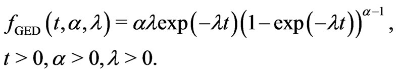
Burr [1] introduced twelve families of distributions for modeling lifetime data. Among those families, Burr type X and Burr type XII have received the most attention. The Burr type X distribution is also known as the generalized Rayleigh distribution (GRD). The probability density function (pdf), cumulative distri-bution function (cdf) and hazard function of the two-parameter GRD are defined, respectively, as below:
 (1.1)
(1.1)
 (1.2)
(1.2)
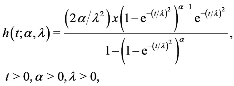 (1.3)
(1.3)
where  is the shape parameter and
  is the scale parameter. If
 , the GRD reduces to the Rayleigh distribution. The GRD has been studied in many papers such as [2-11]. Johnson et al. [12] provided an excellent review for the GRD up to the year of 1995.
When , the GRD has a decreasing pdf (1.1) and a bathtub-type hazard function. When
 , the pdf (1.1) is a right-skewed unimodal function and the hazard function is an increasing function. The twoparameter GRD has several properties commonly happened in the two-parameter gamma, Weibull and generalized exponential distributions. However, when
 , the hazard function (1.3) behaves more close to the hazard function of Weibull with shape parameter greater than 1. Similar to the generalized exponential distribution and Weibull distribution, the GRD has a closed form of cdf and is very popular for dealing with censored data. Readers can refer to [5] and [7] for more detailed information about the comparison among these distributions.
According to complete samples, Surles and Padgett [10] showed that the two-parameter GRD is quite effectively in modeling strength data and general lifetime data. Kundu and Raqab [5] studied many different estimation methods for the GRD. However, it is very often that objects are lost or withdrawn before failure or the object’s lifetime is only known within an interval in industrial life testing applications or medical survival analysis. Hence, the sample information is imcomplete and the obtained sample is called a censored sample. The most common censoring schemes are type-I censoringtype-II censoring and progressive censoring. The life testing is ended at a pre-scheduled time for the type-I censoring and for the type-II, the life testing is ended whenever the number of lifetimes is reached. Both the type-I and the type-II censoring schemes allow withdrawing the test items only at the end of life testing. However, the progressive censoring schemes allow removing test items at some other times before the end of life testing. More information about progressive type-I and type-II censoring schemes and their applications can be found in [13].
Aggarwala [14] introduced the statistical inference procedure for progressively type-I interval censored data from the exponential distribution. Under progressive type-I interval censoring, observations are only known within two consecutively pre-scheduled times and items would be allowed to withdraw at pre-scheduled time points. Ng and Wang [15] studied parameter estimations for Weibull distribution under progressive type-I interval censoring. Chen and Lio [16] inferred the parameters of GED according to progressively type-I interval censored samples. To our best knowledge, there no any research work about the statistical inference for the GRD based on progressively type-I interval censored samples has been published in literatures.
The rest of this article is organized as follows. In Section 2, we introduce the progressive type-I interval censoring scheme into the GRD followed by the theoretical backgrounds and methods for its parameter estimation. A simulation study is conducted in Section 3 to compare the performance of these estimation methods in terms of the mean squared error (MSE) and bias. In Section 4, the application to a real data set is discussed. Some conclusions are given in Section 5.
2. Data, Likelihood and Parameter Estimations
2.1. Progressively Type-I Interval Censored Data
Let  items are placed on a life test simultaneously at the initial time
  and under inspection at
  pre-specified times
 , where
  is the scheduled time to terminate the experiment. At the time
 , the number,
  , of failures occurred in
  is recorded and
  surviving items are randomly removed from the life test, for
 . At the time
 , all surviving items are removed and the life test is terminated. Since the number,
  , of surviving items in
  is a random variable and
  at schedule time
 ,
,  could be determinated by the pre-specified percentage of the remaining surviving units at the time
 . For example, given pre-specified percentage values,
  and
and , for withdrawing at
 , respectively,
  at each inspection time
  where
where . Therefore, a progressively type-I interval censored sample can be denoted as
 , where sample size
 . If
. If , then the progressively type-I interval censored sample is a conventional type-I interval censored sample.
2.2. Likelihood Function
Given a progressively type-I interval censored sample,  , of size
 , from a continuous lifetime distribution with cdf,
  , where
  is the parameter vector, the likelihood function can be constructed as follows (see for example, [1]):
 (2.1)
(2.1)
It can be seen easily that if , the likelihood function (2.1) reduces to the corresponding likelihood function for the conventional type-I interval censoring. The maximum likelihood estimate (MLE) for the parameter can be carried out by maximizing the likelihood function of (2.1). Generally, it is often the case without a closed form for the MLE and therefore an iterative numerical search could be used to obtain the MLE from the above likelihood function.
2.3. Maximum Likelihood Estimation
Given a progressively type-I interval censored sample from the GRD defined by Equation (1.1) and Equation (1.2), the likelihood function, (2.1), can be specified as follows:
 (2.2)
(2.2)
Let . By setting the derivatives of the log likelihood function with respect to
  or
or  to zero, the MLEs of
  and
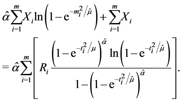
and  are the solutions to the following likelihood equations
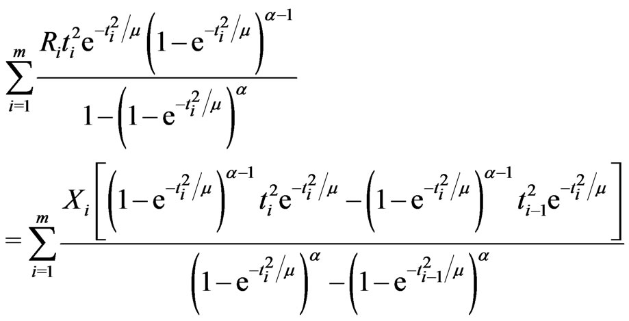 (2.3)
(2.3)
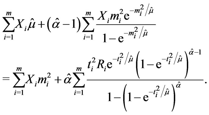
and
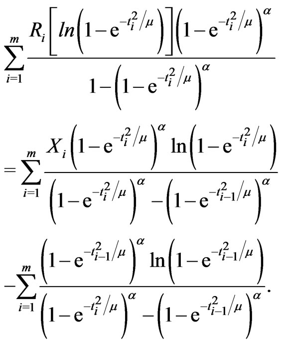 (2.4)
(2.4)
No closed form of the solution can be found to the above equations, and an iterative numerical search can be used to obtain the MLEs. Let  and
and  be the solution to the above equations. Then the MLE for
  is
is . When
  is known and
  is unknown, then only
  needs to be estimated and the MLE is the solution of
  to the Equation (2.4) with
  replaced by the known
 . When
  is known and
  is unknown, then only
  needs to be estimated and the MLE of
  is the positive squared root of the solution,
  to Equation (2.3) with
  replaced by the known
 . Since there is no closed form of the MLE, a mid-point approximation and the Expectation-Maximization (EM) algorithm are introduced as follows for finding the MLEs of
  and
and .
.
2.4. Mid-Point Approximation Method
Suppose that the  failure units in each subinterval
  occurred at the center of the interval
 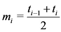 and
and  censored items withdrawn at the censoring time
 . Then the log likelihood function from the GRD could be approximately represented in terms of pseudo-complete data as:
 (2.5)
(2.5)
When  and
and  are unknown, the MLEs,
  and
and , of
, of  and
and  are the solution to the following system of equations,
 (2.6)
(2.6)
and
 (2.7)
(2.7)
Then the estimate for  is
is . When
  is known and
  is unknown, then only
  needs to be estimated and the MLE via mid-point approximation is the solution of
  to the Equation (2.6) with
  replaced by
 . When
  is known and
  is unknown, then only
  needs to be estimated and the MLE of
  via mid-point approximation is the positive squared root of the solution,
  to Equation (2.7) with
  replaced by
 . Again, there is no closed form for the solution and an iterative numerical search is needed to obtain the parameter estimates,
  and
and , from the above equation(s). Thereafter, the estimates are referred as “MidPt” in this paper. Although there is no closed form of solution, the mid-point likelihood equations are simpler than the original likelihood equations.
2.5. EM-Algorithm
The EM algorithm is a broadly applicable approach to the iterative computation of MLEs and useful in a variety of incomplete-data problems where algorithms such as the Newton-Raphson method may turn out to be more complicated. On each iteration of the EM algorithm, there are two steps called the expectation step or the E-step and the maximization step or the M-step. Therefore, the algorithm is called the EM algorithm and the detail development of EM algorithm can be found in [17]. The EM algorithm for finding the MLEs of parameters in the two-parameter GRD is developed as follows.
Let , be the survival times within subinterval
  and
and  be the survival times for those withdrawn items at
  for
for , then the log likelihood,
  , for the complete lifetimes of
  items from the two-parameter GRD is given as follows:
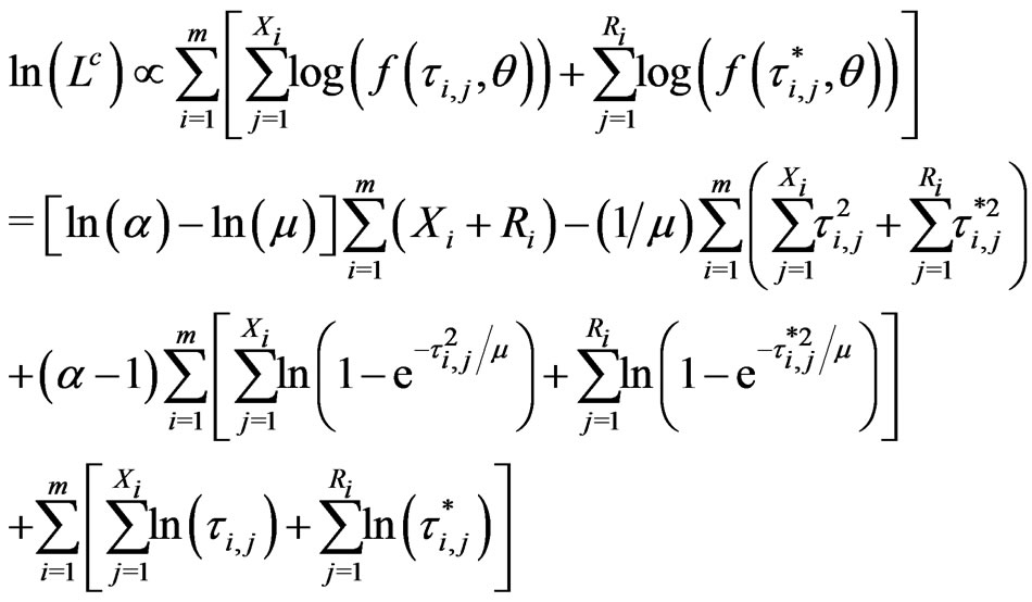 (2.8)
(2.8)
where .
.
Taking the derivative with respective to  and
and , respectively, on Equation (2.8), the following likelihood equations are obtained:
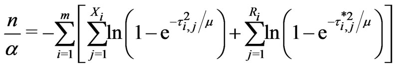 (2.9)
(2.9)
and
 (2.10)
The lifetimes of the  failures in the
  th interval
  are independent and follow a doubly truncated GRD from the left at
  and from the right at
  and the lifetimes of the
  censored items in the
  th interval
  are independent and follow a truncated GRD from the left at
 ,
, . The required expected values of a doubly truncated from the left at
  and from the right at
  with
with  for EM algorithm are given by

Therefore the EM algorithm is given in this case by the following iterative process:
1. Given starting values of ,
,  and
and , say
, say
 ,
,  and
and . Set
. Set .
.
2. In the  th iteration
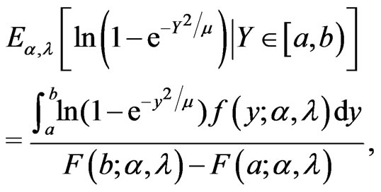
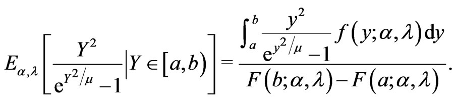
• the E-step requires to compute the following conditional expectations using numerical integration methods,
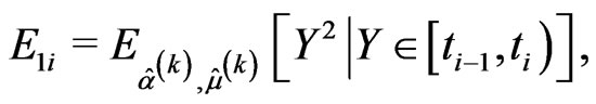
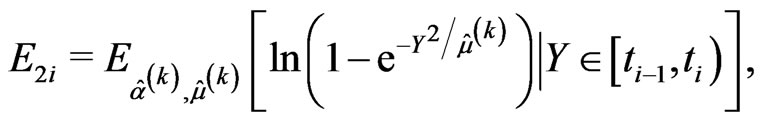
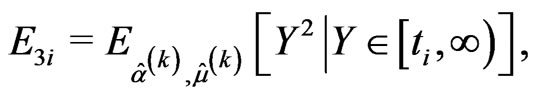
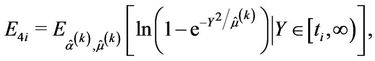

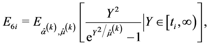
and the likelihood Equations (2.9) and (2.10) are replaced by
 (2.11)
and
 (2.12)
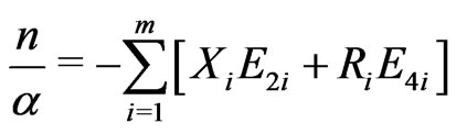
• The M-step requires to solve the Equations (2.11) and (2.12) and obtains the next values,  ,
, 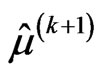 and
and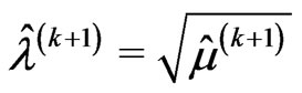 , of
, of ,
,  and
and respectively, as follows:
 (2.13)
 (2.14)
3. Checking convergence, if the convergence occurs then the current ,
,  and
and  are the approximated MLEs of
 ,
,  and
and  via EM algorithm; otherwise, set
  and go to Step 2.
The approximated MLEs of ,
,  and
and  via EM algorithm are thereafter referred as “EM” in this paper. It can be easily seen that the EM algorithm has no complicated likelihood equations involved for solving the solutions as the MLEs of
  and
and . Therefore, it can be efficiently implemented through a computing program.
When  is known and
  is unknown, only
  needs to be estimated and Equation (2.11) and Equation (2.13) with
  replaced by
  will be implemented via EM algorithm to obtain the MLE of
 . Similarly, when
  is known and
  is unknown, only
  needs to be estimated and Equation (2.12) and Equation (2.14) with
  replaced by
  will be implemented via EM algorithm to obtain the MLE of
 .
.
2.6. Method of Moments
Let  be random variable which has the pdf (1.1). Kundu and Raqab [5] and Raqab and Kundu [7] had shown that:


where  is the digamma function and
  is the derivative of
 . The
. The  th moment of a doubly truncated GRD in the interval
  with
with  is given by
Equating the sample moments to the corresponding papulation moments, the following equations can be used to find the estimates of moment method.
 (2.15)
 (2.16)
Since no closed form of the solutions to Equation (2.15) and Equation (2.16) can be obtained, an iterative numerical process to obtain the parameter estimates is described as follows:
1) Let the initial estimates of ,
,  and
and , say
, say
 ,
, and
and  with
with .
.
2) In the  th iteration
• computing ,
,
 ,
,
 and
and
 and solving the following equation for
 , say
, say :
:
 (2.17)
• The solution for , say
, say , is obtained through the following equation
 (2.18)
and 
3) Checking convergence, if the convergence occurs then the current  and
and  are the estimates of
  and
and  by the method of moments; otherwise set
  and go to Step 2. The resultant estimates of
  and
and  is thereafter referred as “MME” in this paper.
When  is known and
  is unknown, estimate
  only using Equation (2.17) with
  replaced by
  will be implemented through the iterative process of the Method of Moments to obtain the “MME” of
 . Similarly, when
  is known and
  is unknown, estimate
  only using Equation (2.18) with
  replaced by
  will be implemented through the iterative process of the Method of Moment to obtain the “MME” of
 .
.
2.7. Estimation Based on Probability Plot
Given a progressively type-I interval censored data,  of size
 , the distribution function at time
  can be estimated by the product-limit distribution described as
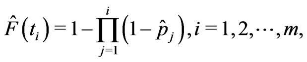 (2.19)
where

From (1.2), we have
 (2.20)
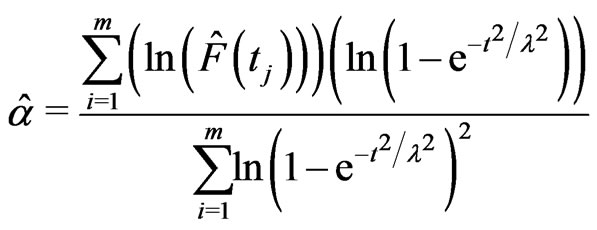
Let  be the estimate of
 , then the estimates of
  and
and  in the GRD based on probability plot can be obtained by minimizing
 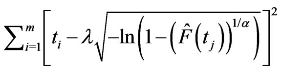 with respect to
  and
and . A nonlinear optimization procedure will be applied here to find the minimizers as the estimates of
  and
and . And the minimizers are thereafter referred as “ProbPt” in this paper.
When  is known and
  is unknown, it can be shown that the estimate,
  of
of  via probability plot is
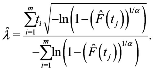 (2.21)
when  is known and
  is unknown, then
 , then the estimate of
 through probability plot can be obtained by minimizing
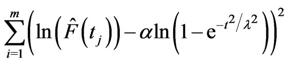 (2.22)
with respect to  and the estimate of
  is
is
 (2.23)
3. Simulation Study
The purpose for simulation study is to investigate the behavior of the proposed estimation methods for the GRD parameters by using progressive type-I interval censored data. Four different simulation schemes are proposed to generate the progressively type-I interval censored data from the GR distribution and the comparison among all estimation processes described in Section 2 will be discussed. The simulation is conducted in R language (R Development Core Team [18]), which is a non-commercial, open source software package for statistical computing and graphics that was originally developed by Ihaka and Gentleman [19]. The R codes can be obtained from the authors upon request.
3.1. Simulation Algorithm
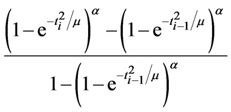
According to the algorithm proposed in [1], a progressively type-I interval censored data,  , from the GRD of (1.1) and (1.2) can be generated as follows: let
  and
and  and for
 ,
,
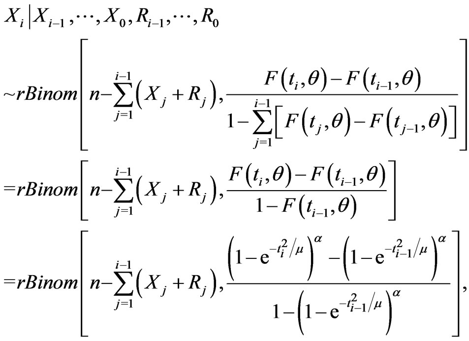 (3.1)
(3.1)
 (3.2)
(3.2)
where  returns the largest integer not greater than the argument. Notice that if
 , then
  and hence
  is a simulated sample from the conventional type-I interval censoring. This algorithm, which is an extension for the procedures in [20] developed for the multinomial distribution, involves to generate
  binomial random variables with the pseudo-code in this case as follows:
1) Set  and let
 .
.
2) 
• Generate  as a binomial random variable with parameters
  and
and
• Calculate
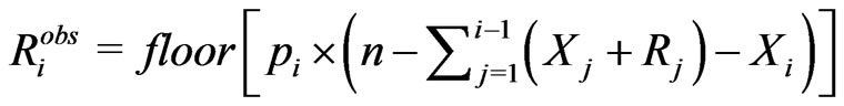 or
or
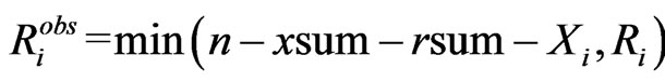 depending upon the censoring scheme implemented by percentage,
  , or
, or .
.
3) Set  and
and .
.
4) If , go to Step 2; otherwise, stop.
3.2. Simulation Schemes
For simplicity, we consider the simulation setups parallel to the real data, given in Section 4, for the  prespecified inspection times in terms of year,

 and
and  which is the time to terminate the experiment. We perform intensive simulations to compare the performance of the different estimators, described in Section 2.
Each replication of the simulation generates a progressively type-I interval censored sample of size  from the GRD with parameters
  in Equation (1.1) and Equation (1.2), both input parameters are selected close to the MLEs of parameters in the GRD for the given data in Section 4.
To compare the performances of the estimation procedures developed in this paper, we consider the following four progressive interval censoring schemes which are similar to the patterns of simulation schemes used in [14], [15] and [16]:

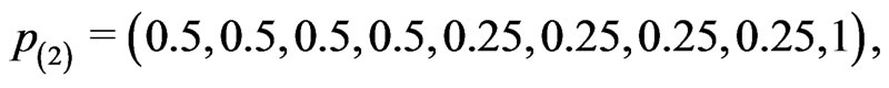
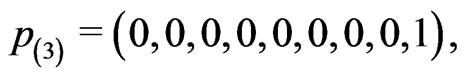
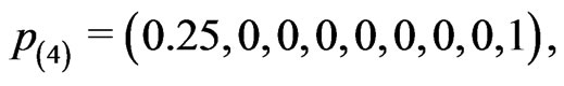
where censoring in  is lighter for the first four intervals and heavier for the next four intervals. The censoring pattern is reversed in
  and
and  is the conventional interval censoring where no removals prior to the experiment termination and the censoring in
  only occur at the left-most and the right-most. The initial values of
  and
and  for iterative progresses of MLE, mid-point approximation, EM algorithm, momemt method and probability plot are given the same value, which is randomly generated, for each simulation run.
3.3. Simulation Results
For given simulation parameter inputs, the simulation is conducted 1000 simulation runs. The median, mean, the absolute value of bias, standard deviation and mean squared error are calculated based on the 1000 MLEs from these 1000 simulation runs. Table 1 sumarizes the simulation results for estimating both unknown GRD parameters. In general, Table 1 indicates that the processes of the regular MLE and EM algorithm give relatively more accurate estimates than the other processes in view of the “Median” and “Mean” in the table although there is a slightly bias as indicated in “Bias” (i.e. the bias). This conclusion can also be supported by Figures 1 and 2 where the medians of the boxplots for the processes of the regular MLE and EM algorithm are close to the input population parameters, 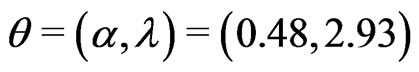 , for the simulation study. However, the boxplots shows that almost all the plots are right skewed except the cases of the plots for the regular MLEs and the MLEs via midpoint approximation for
  under the progressive interval censoring schemes of
  and
and . The box plots also show potential outliers happened for many cases except the case from EM algorithm under progressive censoring scheme
 . It could be due to the convergence problem from the iterative process that outliers happen. Over all, from the box plots, we can conclude that process via EM algorithm provides the best convergence results.
As the performances among the four censoring schemes, the third scheme  provides the most precise results as seen from “Bias”, “SD” (i.e. the standard deviation) and “MSE” (i.e. the mean squared errors) shown in Table 1, then followed by the schemes
 ,
,  or
or . The results of the performance comparisons among these censoring schemes are similar to the results observed in [15] and [16]. These phenomena are expected since the third censoring scheme could have the largest number of failure items observed before the termination of life-testing and then followed by
 ,
,  and
and . Intuitively, these are also consistent with the statistical theory that the larger the “sample size” is the more accuracy the parameter estimate is.
Among these three estimators developed in the paper, the maximum likelihood estimator (via regular process and EM algorithm in the paper) gives the most precise parameter estimates as shown by SD and MSE in Table 1. Therefore, we recommend the maximum likelihood estimation. Among the three processes, “MLE” “MidPt” and “EM”, for the maximum likelihood estimate, “MidPt” has largest “Bias” and comparative “SD” and slightly larger “MSE”. Since the process of EM algorithm provides better convergence results, the MLE via EM algorithm is suggested to be used for the GRD modelling under the progressive type-I interval censoring.
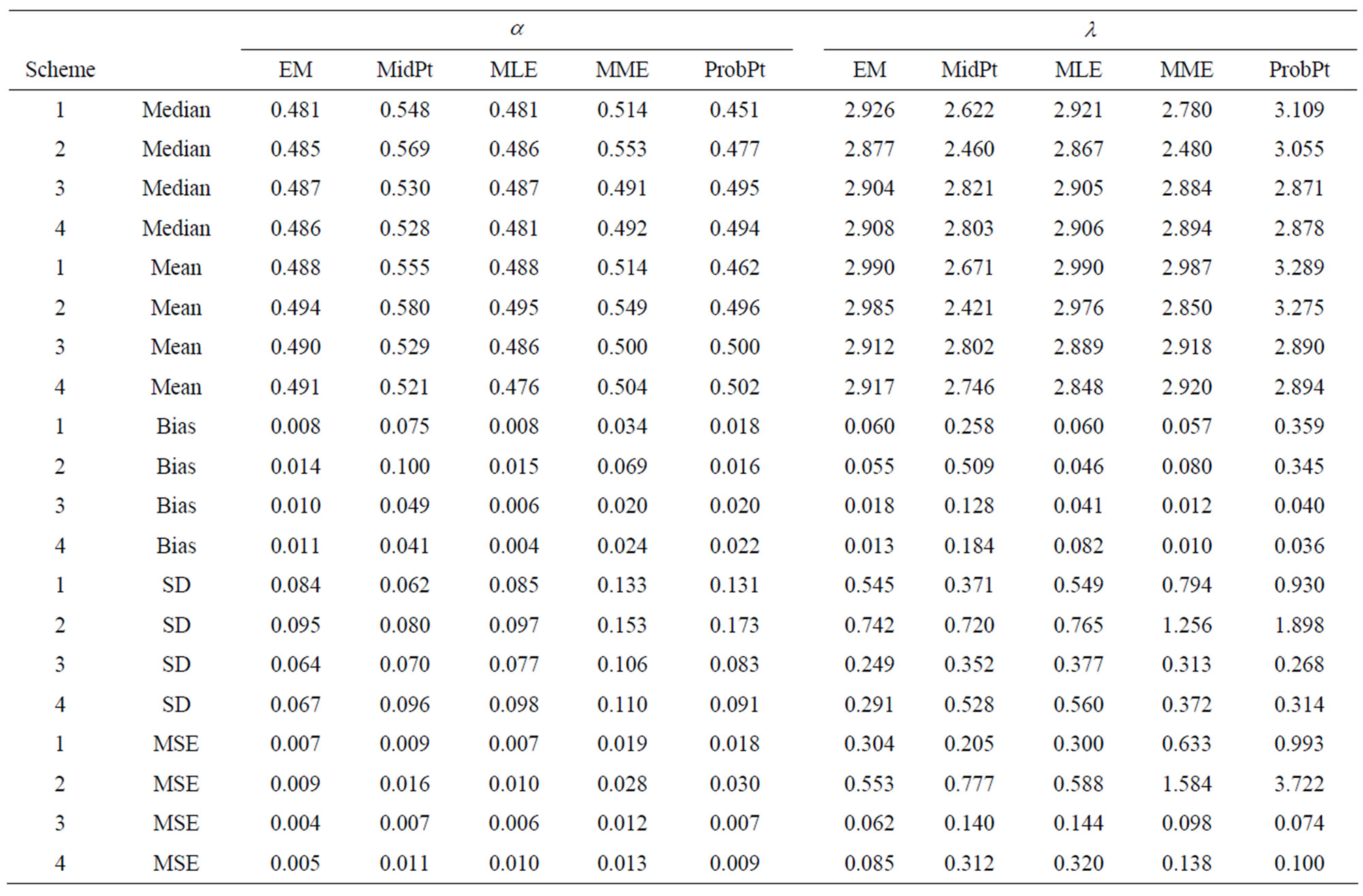
Table 1. Summary of simulations assuming both  and
and  unknown.
4. Real Data Analysis
4.1. The Data
A data set which consists of 112 patients with plasma cell myeloma treated at the National Cancer Institute (See [21]) is used for modelling the two-parameter GRD. This data had been discussed in [15], [16] and [22]. To be self-contained, the data are re-produced here in the Table 2 for easy reference.
The most right side column in Table 2 shows the number of patients who were dropped out from the study at the right end of each time interval. These dropped patients are known to be survived at the right end of each time interval but no follow-up. Hence, the most right side column in Table 2 provides the values of . The number of failures,
  , can be easily calculated to be
  from the number at risk and the number of withdrawals.
4.2. Model Comparisons
Weibull distribution from [15] and generalized exponential distribution from [16] have been used to model the plasma cell myeloma data set with prescheduled times in terms of month. Chen and Lio [16] also compare the modelling processes between Weibull distribution and generalized exponential distribution by using prescheduled times in terms of month. Chen and Lio [16] indicated that the generalized exponential distribution provided better model fit than the Weibull distribution does. In this paper, we would like to compare the modelling processes among Weibull distribution, generalized exponential distribution and generalized Rayleigh distribution. To compare the modelling processes among these three distributions, the prescheduled times are converted into in terms of year. Here, it is for easy reference that the pdfs of Weibull distribution and generalized exponential distribution are given, respectively, below:
 (4.1)
(4.1)
and
 (4.2)
(4.2)
The model fitting to the classical Weibull distribution (1) yields the estimated parameters
 and log likelihood,

Table 2. Plasma cell myeloma survival times.
has  and the model fitting to the generalized exponential distribution (2) has the estimated parameters
  and log likelihood,
  has
has  . The model fitting results for both Weibull distribution and generalized exponential distribution reported here are different from the results reported in [16]. For the GRD model fitting, the estimated parameters are
  and log likelihood,
  has
has  . It could be seen that all three maximum likelihood values for these probability modelling processes are virtually identical. Since all these

Figure 1. Boxplot for  from 1000 simulations for the five estimation methods and four simulation schemes for
 .
.

Figure 2. Boxplot for  from 1000 simulations for the five estimation methods and four simulation schemes for
 .
.
three distributions have no sub-model relationship, the chi-square test can not be applied directly to select among these three models for modeling the given data set. Although Kundu and Raqab [5] and Raqab and Kundu [7] had detail comparison among these distribution for a random sample, statistical inference to discriminate among these distributions has not been developed for the progressively type-I interval censored data, yet. Therefore, a more detail comparison among these three distributions under progressive type-I interval censoring is not available according to our best knowledge.
To apply the Kolmogorov-Smironov goodness-of-fit test for fitting a given complete data set with a distribution,  , the maximum distance,
 , between the empirical distribution,
  , of the given data set and the population distribution,
  with
with  as the MLE of
 , must be obtained. When a progressively censored data is given, the empirical distribution is replaced by the product-limit distribution defined through Equation (19) in the formula
 . Fitting the given data set with the Weibull distribution
 ,
,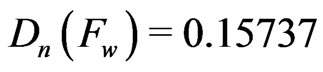 , with the GE distribution
 ,
, 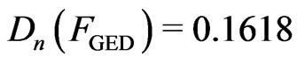 and with the GRD
 ,
,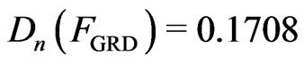 . Again, the reports of the Kolmogorov-Smironov goodness-of-fit test for the Weibull distribution and generalized exponential distribution are different from the reports of [16]. The sampling distribution of
  should have been applied to find the critical value for the goodness-of-fit tests mentioned. Although the sampling distribution for
  under any progressive censoring has not been developed, we can see that no any significant difference among these three numerical reports.
5. Discussions and Conclusions
In this paper, three methods to estimate the parameters of the two-parameter generalized Rayleigh distribution under progressive type-I interval censoring have been developed. They are maximum likelihood estimation, estimation of method moments and the estimation based on the probability plot.
The simulation study in the case of moderate large size data set indicates that regular MLE and maximum likelihood estimate via EM algorithm gives relatively more accurate parameter estimation and the maximum likelihood estimate via EM algorithm produces the most precise estimation as summarized in the Table 1 and Figures 1 and 2. We therefore recommend the EM algorithm process to be used to estimate the parameters in the GRD under progressive type-I interval censoring.
The developed methods are also applied to a real data which contains 112 patients with plasma cell myeloma treated at the National Cancer Institute to demonstrate the applicability. In the process of GRD modelling, it is found that the value of likelihood function (2.2) closes to zero when the prescheduled times in terms of month and the estimations of parameters are senstive to the initial parameter inputs for iterative processes. Many rescales for the prescheduled times have been tried. We found that the prescheduled times must be converted into in terms of year to produce better convergence results in the propulation parameter estimations. The parameter estimates for the GRD via EM algorithm and regular MLE are quite similar. This real data set modelling confirms the results observed from the simulation study.
Since the GRD was introduced for lifetime data, this study was the first time to introduce the progressive type-I interval censoring to the GRD based on our best knowledge. We believe that this study contributes to the literatures and the research community in this lifetime data analysis for the generalized Rayleigh distribution as well as for progressive type-I interval censoring.
The comparison among Weibull distribution, generalized exponential distribution and generalized Rayleigh distribution in the modelling process for the progressively type-I interval censored data shows that no much difference among these three modelling processes. Hence, the discriminate process among these three distibutions under progressive type-I censoring could be an important future research.
6. Acknowledgements
The authors would like thank to the editor and anonymous referees for their suggestions and comments, which significantly improved this manuscript.
7. References
[1] I. W. Burr, “Cumulative Frequency Distribution,” Annual of Mathematical Statistics, Vol. 13, No. 2, 1942, pp. 215-232.
[2] K. E. Ahmad, M. E. Fakhry and Z. F. Jaheen, “Empirical Bayes Estimation of P (Y < X) and Characterization of Burr-Type X Model,” Journal of Statistical Planning and Inference, Vol. 64, No. 2, 1997, pp. 297-308. doi:10.1016/S0378-3758(97)00038-4
[3] Z. F. Jaheen, “Bayesian Approach to Prediction with Outliers from the Burr Type X Model,” Microeleclron Reliability, Vol. 35, No. 4, 1995, pp. 45-47. doi:10.1016/0026-2714(94)00056-T
[4] Z. F. Jaheen, “Empirical Bayes Estimation of the Reliability and Failure Rate Functions of the Burr Type X Failure Model,” Journal Applied Statistical Science, Vol. 3, No. 2, 1996, pp. 281-285.
[5] D. Kundu and M. Z. Raqab, “Generalized Rayleigh Distribution: Different Methods of Estimation,” Computational Statistics and Data Analysis, Vol. 49, No. 1, 2005, pp. 187-200. doi:10.1016/j.csda.2004.05.008
[6] M. Z. Raqab, “Order Statistics from the Burr Type X Model,” Computational Mathematical Applications, Vol. 36, No. 4, 1998, pp. 111-120. doi:10.1016/S0898-1221(98)00143-6
[7] M. Z. Raqab and D. Kundu, “Burr Type X Distribution: Revisited,” 2003. http://home.iitk.ac.in/ kundu/paper118.pdf
[8] H. A. Sartawi and M. S. Abu-Salih, “Bayes Prediction Bounds for the Burr Type X Model,” Communication in Statistics: Theory and Methods, Vol. 20, No. 7, 1991, pp. 2307-2330. doi:10.1080/03610929108830633
[9] J. Q. Surles and W. J. Padgett, “Inference for P(Y < X) in the Burr Type X Model,” Journal Applied Statistical Science, Vol. 7, No. 2, 1998, pp. 225-238.
[10] J. Q. Surles and W. J. Padgett, “Inference for Reliability and Stress-Strength for a Scaled Burr Type X Model,” Lifetime Data Analysis, Vol. 7, No. 2, 2001, pp. 187-200. doi:10.1023/A:1011352923990
[11] J. Q. Surles and W. J. Padgett, “Some Properties of a Scaled Burr Type X Model,” Joournal Statisticsal Planning and Inference, Vol. 7, No. 2, 2004, pp. 187-200.
[12] N. L. Johnson, S. Kotz and N. Balakrishnan, “Continuous Univariate Distribution,” Vol. 1, 2nd Edition, John Wiley and Sons, New York, 1995.
[13] N. Balakrishnan and R. Aggarwala, “Progressive Censoring: Theory, Methods and Applications,” Birkha User, Boston, 2000.
[14] R. Aggarwala, “Progressively Interval Censoring: Some Mathematical Results with Application to Inference,” Communications in Statistics-Theory and Methods, Vol. 30, No. 8, 2010, pp. 1921-1935.
[15] H. Ng and Z. Wang, “Statistical Estimation for the Parameters of Weibull Distribution Based on Progressively type-I Interval Censored Sample,” Journal of Statistical Computation and Simulation, Vol. 79, No. 2, 2009, pp. 145-159. doi:10.1080/00949650701648822
[16] D. G. Chen and Y. L. Lio, “Parameter Estimations for Generalized Exponential Distribution under Progressive Type-I Interval Censoring,” Computational Statistics and Data Analysis, Vol. 54, No. 6, 2010, pp. 1581-1591. doi:10.1016/j.csda.2010.01.007
[17] A. P. Dempster, N. M. Laird and D. B. Rubin, “Maximum Likelihood from Incomplete Data via the EM Algorithm,” Journal of the Royal Statistical Society: Series B, Vol. 39, No. 1, 1977, pp. 1-38.
[18] R Development Core Team, “A Language and Environment for Statistical Computing,” R Foundation for Statistical Computing, Vienna, 2006.
[19] R. Ihaka and R. Gentleman, “R: A Language for Data Analysis and graphics,” Journal of Computational and Graphical Statistics, Vol. 5, No. 3, 1996, pp. 299-314. doi:10.2307/1390807
[20] C. D. Kemp and W. Kemp, “Repid Generation of Frequency Tables,” Applied Statistics, Vol. 36, No. 3, 1987, pp. 277-282. doi:10.2307/2347786
[21] P. P. Carbone, L. E. Kellerhouse and E. A. Gehan, “Plasmacytic Myeloma: A Study of the Relationship of Survival to Various Clinical Manifestations and Anomalous Protein Type in 112 Patients,” The American Journal of Medince, Vol. 42, No. 6, 1967, pp. 937-948. doi:10.1016/0002-9343(67)90074-5
[22] J. Lawless, “Statistical Models and Methods for Lifetime Data,” John Wiley and Sons, New York, 1982.