American Journal of Computational Mathematics
Vol.4 No.2(2014), Article ID:43977,18 pages DOI:10.4236/ajcm.2014.42006
An Actual Survey of Dimensionality Reduction
Alireza Sarveniazi
Institut fuer Angewandte Forschung (IAF), Karlsruhe, Germany
Email: alireza.sarveniazi@hs-karlsruhe.de
Copyright © 2014 by authors and Scientific Research Publishing Inc.
This work is licensed under the Creative Commons Attribution International License (CC BY).
http://creativecommons.org/licenses/by/4.0/


Received 6 November 2013; revised 6 December 2013; accepted 15 December 2013
ABSTRACT
Dimension reduction is defined as the processes of projecting high-dimensional data to a much lower-dimensional space. Dimension reduction methods variously applied in regression, classification, feature analysis and visualization. In this paper, we review in details the last and most new version of methods that extensively developed in the past decade.
Keywords:Dimensionality Reduction Methods

1. Introduction
Any progresses in efficiently using data processing and storage capacities need control on the number of useful variables. Researchers working in domains as diverse as computer science, astronomy, bio-informatics, remote sensing, economics, face recognition are always challenged with the reduction of the number of data-variables. The original dimensionality of the data is the number of variables that are measured on each observation. Especially when signals, processes, images or physical fields are sampled, high-dimensional representations are generated. High-dimensional data-sets present many mathematical challenges as well as some opportunities, and are bound to give rise to new theoretical developments [1] .
In many cases, these representations are redundant and the varaibles are correlated, which means that eventually only a small sub-space of the original representation space is populated by the sample and by the underlying process. This is most probably the case, when very narrow process classes are considered. For the purpose of enabling low-dimensional representations with minimal information loss according dimension reduction methods are needed.
Hence, we are reviewing in this paper the most important dimensional reduction methods, including most traditional methods, such as principal component analysis (PCA) and non-linear PCA up to current state-of-art methods published in various areas, such as signal processing and statistical machine learning literature. This actual survey is organized as follows: section 2 reviews the linear nature of Principal component analysis and its relation with multidimensional scaling (classical scaling) in a comparable way. Section 3 introduces non-linear or Kernel PCA (KPCA) using the kernel-trick. Section 4 is about linear discriminant analysis (LDA), and we give an optimization model of LDA which is a measuring of a power of this method. In section 5 we summarize another higher-order linear method, namely canonical correlation analysis (CCA)), which finds a low dimensional representation maximizing the correlation and of course its optimization-formulation. Section 6 reviews the relatively new version of PCA, the so-called oriented PCA (OPCA) which is introduced by Kung and Diamantaras [2] as a generalization of PCA. It corresponds to the generalized eigenvalue decomposition of a pair of covariance matrices, but PCA corresponds to the eigenvalue decomposition of only a single covariance matrix. Section 7 introducs principal curves and includes a characterization of these curves with an optimization problem which tell us when a given curve can be a principal curve. Section 8 gives a very compact summary about non-linear dimensional-reduction methods using neural networks which include the simplest neural network which has only three layers:
1) Input Layer 2) Hidden Layer (bottleneck)
3) Output Layer and an auto-associative neural network with five layers:
1) Input Layer 2) Hidden Layer 3) Bottleneck 4) Hidden Layer 5) Output Layer A very nice optimizing formulation is also given. In section 9, we review the Nystroem method which is a very useful and well known method using the numerical solution of an integral equation. In Section 10, we look the multidimensional scaling (MDS) from a modern and more exact consideration view of point, specially a defined objective stress function arises in this method. Section 11 summarizes locally linear embedding (LLE) method which address the problem of nonlinear dimensionality reduction by computing low-dimensional neighborhood preserving embedding of high-dimensional data. Section 12 is about one of the most important dimensional-reduction method namely Graph-based method. Here we will see how the adjacency matrix good works as a powerful tool to obtain a small space which is in fact the eigen-space of this matrix. Section 13 gives a summary on Isomap and the most important references about Dijstra algorithm and Floyd’s algorithm are given. Section 14 is a review of Hessian eigenmaps method, a most important method in the so called manifold embedding. This section needs more mathematical backgrounds. Section 15 reviews most new developed methods such as
• vector quantization
• genetic and evolutionary algorithms
• regression We have to emphasize here the all of given references in the body of survey are used and they are the most important references or original references for the related subject. To obtain more mathematical outline and sensation, we give an appendix about the most important backgrounds on the fractal and topological dimension definitions which are also important to understand the notion of intrinsic dimension.
2. Principal Component Analysis (PCA)
Principal component Analysis (PCA) [3] [4] [5] -[8] is a linear method that it performs dimensionality reduction by embedding the data into a linear subspace of lower dimensional. PCA is the most popular unsupervised linear method. The result of PCA is a lower dimensional representation from the original data that describes as much of the variance in the data as possible. This can be reached by finding a linear basis (possibly orthogonal) of reduced dimensionality for the data, in which the amount of variance in the data is maximal.
In the mathematical language, PCA attempts to find a linear mapping  that maximizes the cost function
 , where
  is the sample covariance matrix of the zero-mean data. Another words PCA maximizes
  with respect to
  under the constraint the norm of each column
  of
of  is
is , i.e.,
 . In fact PCA solves the eigenvalue problem:
![]() (1.1)
(1.1)
Why the above optimization Problem is equivalent to the eigenvalue problem (1.1)? consider the convex form , it is a straightforward calculation that the maximum happens when
![]() .
.
It is interesting to see that in fact PCA is identical to the multidimensional scaling (classical scaling) [9] .
For the given data  let
let  be the pairwise Euclidean matrix whose entries
  represent the Euclidean distance between the high-dimensional data points
  and
and . multidimensional scaling finds the linear mapping
  such that maximizes the cost function:
 (1.2)
(1.2)
in which  is the Euclidean distance between the low-dimensional data points
  and
and ,
,  is restricted to be
![]() , with
, with  for all column vector
  of
of . It can be shown [10] [11] that the minimum of the cost function
  is given by the eigen-decomposition of the Gram matrix
  where
where . Actually we can obtain the Gram matrix by double-centering the pairwise squared Euclidean distance matrix, i.e., by computing:
 (1.3)
(1.3)
Now consider the multiplication of principal eigenvectors of the double-centered squared Euclidean distance matrix (i.e., the principal eigenvectors of the Gram matrix) with the square-root of their corresponding eigenvalues, this gives us exactly the minimum of the cost function in Equation (1.2).
It is well known that the eigenvectors  and
and  of the matrices
  and
and  are related through
![]() [12] , it turns out that the similarity of classical scaling to PCA . The connection between PCA and classical scaling is described in more detail in, e.g., [11] [13] . PCA may also be viewed upon as a latent variable model called probabilistic PCA [14] . This model uses a Gaussian prior over the latent space, and a linearGaussian noise model.
[12] , it turns out that the similarity of classical scaling to PCA . The connection between PCA and classical scaling is described in more detail in, e.g., [11] [13] . PCA may also be viewed upon as a latent variable model called probabilistic PCA [14] . This model uses a Gaussian prior over the latent space, and a linearGaussian noise model.
The probabilistic formulation of PCA leads to an EM-algorithm that may be computationally more efficient for very high-dimensional data. By using Gaussian processes, probabilistic PCA may also be extended to learn nonlinear mappings between the high-dimensional and the low-dimensional space [15] . Another extension of PCA also includes minor components (i.e., the eigenvectors corresponding to the smallest eigenvalues) in the linear mapping, as minor components may be of relevance in classification settings [16] . PCA and classical scaling have been successfully applied in a large number of domains such as face recognition [17] , coin classification [18] , and seismic series analysis [19] .
PCA and classical scaling suffer from two main drawbacks. First, in PCA, the size of the covariance matrix is proportional to the dimensionality of the data-points. As a result, the computation of the eigenvectors might be infeasible for very high-dimensional data. In data-sets in which![]() , this drawback may be overcome by performing classical scaling instead of PCA, because the classical scaling scales with the number of data-points instead of with the number of dimensions in the data. Alternatively, iterative techniques such as Simple PCA [20] or probabilistic PCA [14] may be employed. Second, the cost function in Equation (1.2) reveals that PCA and classical scaling focus mainly on retaining large pairwise distances
, this drawback may be overcome by performing classical scaling instead of PCA, because the classical scaling scales with the number of data-points instead of with the number of dimensions in the data. Alternatively, iterative techniques such as Simple PCA [20] or probabilistic PCA [14] may be employed. Second, the cost function in Equation (1.2) reveals that PCA and classical scaling focus mainly on retaining large pairwise distances![]() , instead of focusing on retaining the small pairwise distances, which is much more important.
, instead of focusing on retaining the small pairwise distances, which is much more important.
3. Non-Linear PCA
Non-linear or Kernel PCA (KPCA) is in fact the reconstruction from linear PCA in a high-dimensional space that is constructed using a given kernel function [21] . Recently , such reconstruction from linear techniques using the kernel-trick has led to the proposal of successful techniques such as kernel ridge regression and Support Vector Machines [22] . Kernel PCA computes the principal eigenvectors of the kernel matrix, rather than those of the covariance matrix. The reconstruction from PCA in kernel space is straightforward, since a kernel matrix is similar to the inner product of the data-points in the high-dimensional space that is constructed using the kernel function. The application of PCA in the kernel space provides Kernel PCA the property of constructing nonlinear mappings.
Kernel PCA computes the kernel matrix  of the data-points
 . The entries in the kernel matrix are defined by
 (1.4)
(1.4)
where  is a kernel function [22] , which may be any function that gives rise to a positive-semi-definite kernel K. Subsequently, the kernel matrix
 ![]() is double-centered using the following modification of the entries
is double-centered using the following modification of the entries
 (1.5)
(1.5)
The centering operation corresponds to subtracting the mean of the features in traditional PCA: it subtracts the mean of the data in the feature space defined by the kernel function . Hence, the data in the features space defined by the kernel function is zero-mean. Subsequently, the principal d eigenvectors
  of the centered kernel matrix are computed. The eigenvectors of the covariance matrix
  (in the feature space constructed by
 ) can now be computed, since they are related to the eigenvectors of the kernel matrix
  (see, e.g., [12] ) through
 (1.6)
(1.6)
In order to obtain the low-dimensional data representation, the data is projected onto the eigenvectors of the covariance matrix . The result of the projection (i.e., the low-dimensional data representation
  is given by:

where ![]() indicates the
indicates the  value in the vector
  and
and  is the kernel function that was also used in the computation of the kernel matrix. Since Kernel PCA is a kernel-based method, the mapping performed by Kernel PCA relies on the choice of the kernel function
 . Possible choices for the kernel function include the linear kernel (making Kernel PCA equal to traditional PCA), the polynomial kernel, and the Gaussian kernel that is given in [12] . Notice that when the linear kernel is employed, the kernel matrix K is equal to the Gram matrix, and the procedure described above is identical to classical scaling (previous section).
An important weakness of Kernel PCA is that the size of the kernel matrix is proportional to the square of the number of instances in the data-set. An approach to resolve this weakness is proposed in [23] [24] . Also, Kernel PCA mainly focuses on retaining large pairwise distances (even though these are now measured in feature space).
Kernel PCA has been successfully applied to, e.g., face recognition [25] , speech recognition [26] , and novelty detection [25] . Like Kernel PCA, the Gaussian Process Latent Variable Model (GPLVM) also uses kernel functions to construct non-linear variants of (probabilistic) PCA [15] . However, the GPLVM is not simply the probabilistic counterpart of Kernel PCA: in the GPLVM, the kernel function is defined over the low-dimensional latent space, whereas in Kernel PCA, the kernel function is defined over the high-dimensional data space.
4. Linear Discriminant Analysis (LDA)
The main Reference here is [27] see also [28] . The LDA is a method to find a linear transformation that maximizes class separability in the reduced dimensional space. The criterion in LDA is in fact to maximize between class scatter and minimize within-class scatter. The scatters are measured by using scatter matrices. Let we have
 class
class ![]() each including
each including  points
 ![]() and set
and set , where
  and
and . Let
. Let  and
and .
.
Now we define three scatter matrices:
The between-class scatter matrix The within-class scatter matrix
 The total scatter matrix
 . Actually LDA is a method for the following optimization problem:

Hence in this way the dimension is reduced from  to
to  by a linear transformation
 ![]() which is the solution of above optimization problem. Although we know from Fukunaga (1990), (see [27] and [29] ) that the eigenvectors corresponding to the
which is the solution of above optimization problem. Although we know from Fukunaga (1990), (see [27] and [29] ) that the eigenvectors corresponding to the  largest eigenvalues of

form the columns of U as above for LDA.
5. Canonical Correlation Analysis (CCA)
CCA is an old method back to the works of Hotelling 1936 [30] , recently Sun et al. [31] used CCA as an unsupervised feature fusion method for two feature sets describing the same data objects. CCA finds projective directions which maximize the correlation between the feature vectors of the two feature sets.
Let  and
and  be two data set of
  points in
  and
and  respectively, associate with them we have two matrices:
![]() ,
, ![]()
where  and
and  are the means of
  and
and  s, respectively.
Actually CCA is a method for the following optimization problem:

which can be modified as
 ,
,  ,
, 
Assume the pair of projective directions  be the solution of above optimization problem, we can find another pair of projective directions by solving
 ,
,  ,
, 
repeating the above process ![]() times we obtain a
times we obtain a  -dimensional specs of linear combination of these vector-solutions.
In fact we can obtain this  -dimensional space with solving of the paired eigenvalue problem:
 ,
, 
and the eigenvectors  corresponding to the
  largest eigenvalues are the pairs of projective directions for CCA see [31] . Hence
 and
and 
compose the feature sets extracted from  and
and  by CCA. It turns out that the number
  is determined as the number of nonzero eigenvalue.
6. Oriented PCA (OPCA)
Oriented PCA is introduced by Kung and Diamantaras [2] as a generalization of PCA. It corresponds to the generalized eigenvalue decomposition of a pair of covariance matrices in the same way that PCA corresponds to the eigenvalue decomposition of a single covariance matrix. For the given pair of vectors  and
and  the objective function maximized by OPCA is given as follows:

where ,
, . A solution
  of above optimization problem is called Principal oriented component and it is the generalized eigenvector of matrix pair
  corresponding to maximum generalized eigenvalue
 . Since
  and
and  are symmetric all the generalized eigenvalues are real and thus they can be arranged in decreasing order, as with ordinary PCA. Hence we will obtain the rest generalized eigenvectors
 , as second , third, ×××,
  oriented principal components. All of these solutions are the solutions under the orthogonality constraint:
![]()
7. Principal Curves and Surfaces
By the definition, principal curves are smooth curves that pass through the middle of multidimensional data sets, see [32] -[34] as main references and also [35] and [36] .
Given the  -dimensional random vector
 ![]() with probability density function
with probability density function . Let
. Let  be the given smooth curve which can be parametrized by a real value
 ![]() (actually we can choose
(actually we can choose ). Hence we have
 .
.
we can associate to the curve ![]() the projection index
the projection index ![]() geometrically as the value of
geometrically as the value of ![]()
corresponding to the point on the curve ![]() that under Euclidean metric is the closet point to
that under Euclidean metric is the closet point to .
.
We say ![]() is self-consistent if each point
is self-consistent if each point  is the mean of all points in the support of density function
 ![]() that are projected on
that are projected on![]() , i.e.,
, i.e.,

It is shown in [32] that the set of principal curves do not intersect themselves and they are self-consistent. Most important fact about principal curves which proved in [32] is a characterization of these curves with an optimization Problem:
Theorem 1 A curve ![]() is a principal curve (associate with the data set
is a principal curve (associate with the data set ) iff it solves fallowing optimization problem
 (1.7)
(1.7)
Of course to solve (or even estimate) minimization (0.7) is a complex problem, to estimate ![]() and
and ![]() in
in
[32] an iterative algorithm has given. It started with , where
  is the first eigenvector of covariance matrix of
  and
and . Then it iterates the two steps:
• For a fixed![]() , minimize
, minimize  by setting
• 
• Fix ![]() and set
and set  for each
  until the change in
  is less than a threshold.
One can find in [37] another formulation of the principal curves, along with a generalized EM algorithm for its estimation under Gaussian pdf . Unfortunately except for a few special cases, it is an open problem for what type of distributions do principal curves exist, how many principal curves there exist and which properties the have see [36] . in recent years the concept of principal curves has been extended to higher dimensional principal surfaces, but of course the estimation algorithms are not smooth as the curves.
8. Non-Linear Methods Using Neural Networks
Given Input variables , neural networks getting this input and gives output variables
  with
with

where the weights  are determined by training the neural network using a set of given instances and a cost function see [38] . Over the last two decades there are several developments based on a ring architectures and learning algorithms of dimensional reduction techniques could be implemented using neural networks, see [35] [36] [38] -[40] . Consider the simplest neural network which has only three layers:
1) Input Layer 2) Hidden Layer (bottleneck)
3) Output Layer there are two steps here:
• In order to obtain the data at node  of the hidden layer, we have to consider any inputs
  in combination with their associated weight’s
  along with a threshold term (or called bias in some references)
 , Now they are ready passing through to the corresponding activation
 , hence we are building up the expression
 .
.
• Here we have to repeat step (1) with changing original data  with new one namely
 , of course according the threshold
  and possibly new output function
![]() . Hence we have:
. Hence we have:

We observe that the first part of network reduces the input data into the lower-dimensional space just as same as a linear PCA, but the second part decodes the reduced data into the original domain [36] [35] . Note that only by adding two more hidden layers with nonlinear activation functions, one between the input and the bottleneck, the other between the bottleneck and the output layer, the PCA network can be generalized to obtain non-linear PCA. One can extend this idea from the feed-forward neural implementation of PCA extending to include non-linear activation function in the hidden layers [41] ,. In this framework, the non-linear PCA network can be considered of as an auto-associative neural network with five layers:
1) Input Layer 2) Hidden Layer 3) Bottleneck 4) Hidden Layer 5) Output Layer If ![]() be the function modeled by layers
be the function modeled by layers ,
,  and
and , and
, and  be the modeled function by layers
 ,
,  and
and , in [35] have been shown that weights of the non-linear PCA network are determined such that the following optimization Problem solved:

As we have seen in the last section the function ![]() must be Principal curve(surface). In the thesis [42] , one can find comparison between PCA, Vector Quantization and five layer neural networks, for reducing the dimension of images.
must be Principal curve(surface). In the thesis [42] , one can find comparison between PCA, Vector Quantization and five layer neural networks, for reducing the dimension of images.
9. Nystroem Method
The Nystroem Method is a well known technique for finding numerical approximations of generic integral equation and specially to eigenfunction problems of the following form:

We can divide the interval  into
into  points
  where
where
 and
and ,
,  ,
, .
.
Now consider the simple quadrature rule:
 (1.8)
(1.8)
which  approximates
 , for
, for  we obtain a system of
  equations:

without loss of generality we can shift interval  to unit interval
  and change the above system of equations to the following eigenvalue problem:
![]() (1.9)
(1.9)
where ,
,  and
and , substituting back into 0.8 yields the Nstroem extension for each
 :
:

We can extend above arguments for  and
and![]() , see [42] .
, see [42] .
Motivated from 0.9 our main question is if  be a given
  real symmetric matrix with small rank
 , i.e.,
  , can we approximate the eigenvectors and eigenvalues of A using those of a small sub-matrix of A?
Nystroem method gives a positive answer to this question. Actually we can assume that the  randomly chosen samples come first and the
  samples come next. Hence the matrix
  in 0.9 can have following form:

Hence  represents the sub-block of weights among the random samples,
  contains the weights from the random samples to the rest of samples and C contains the weights between all of remaining samples. Since
 ,
, ![]() must be a large matrix. Let
must be a large matrix. Let ![]() denote the approximate eigenvectors of
denote the approximate eigenvectors of , the Nystroem extension method gives:

where ![]() and
and ![]() are eigenvectors and diagonal matrix associate with
are eigenvectors and diagonal matrix associate with , i.e.,
 . Now the associated approximation of
 , which we denote it with
 , then we have:

The last equation is called “bottleneck” form. There is a very interesting application of this form in Spectral Grouping which it was possible to construct the exact eigen-decomposition of  using the eigendecomposition of smaller matrix rank
 . Also Fowlkes et al have given an application of the Nystroem method t NCut Problem, see [43] .
10. Multidimensional Scaling (MDS)
Given ![]() point
point ![]() and build up the distance matrix
and build up the distance matrix  where
where ,
,  or in general
  for some metric which defined
  MDS
MDS  better to say a
  -dimensional MDS
  is a technique that produces output points
 ![]() such that the distances
such that the distances  are as close as possible to a function
  of the corresponding proximity's
 . From [36] , whether this function
  is linear or non-linear, MDS is called either metric or non-metric. Define an objective stress function MDS-PROCEDURE:
• Define an objective stress function and stress factor , that it depends on
  or on
or on 
 (1.10)
• Now if for a given ![]() as above, find
as above, find  that minimize 0.10, i.e.•
• Determine the optimal data set ![]() by
by

If we use Euclidean distance and take  in Equation (1.10) the produced output data set should be coincide to the Principal component of cov(X)( without re-scaling to correlation), hence in this special case MDS and PCA are coincide (see [44] ) There exist an alternative method to MDS, namely Fast Map see[45] [46] .
11. Locally Linear Embedding (LLE)
Locally linear embedding is an approach which address the problem of nonlinear dimensionality reduction by computing low-dimensional neighborhood preserving embedding of high-dimensional data. A data set of dimensionality , which is assumed to lie on or near a smooth nonlinear manifold of dimensionality
 , is mapped into a single
  coordinate system of lower-dimensionality
 . The global nonlinear structure is recovered by locally linear fits.As usual given a Data set of
 ![]() points on a
points on a  -dimensional points
  from some underlying manifold. Without loss of generality we can assume each data point and its neighbors lie on are close to a locally linear sub-manifold. By a linear transform, consisting of a translation, rotation and rescaling, the high-dimensional coordinates of each neighborhood can be mapped to global internal coordinates on the manifold. In order to map the high-dimensional data to the single global coordinate system of the manifold such that the relationships between neighboring points are preserved. This proceeds in three steps:
• Identify neighbors of each data point . this can be done by finding the
 ![]() nearest neighbors, or choosing all points within some fixed radius
nearest neighbors, or choosing all points within some fixed radius .
.
• Compute the weights  that best linearly reconstruct
  from its neighbors.
• Find the low-dimensional embedding vector  which is the best reconstructed by the weights determined in the previous step.
After finding the nearest neighbors in the first step, the second step must compute a local geometry for each locally linear sub-manifold. This geometry is characterized by linear coefficients that reconstruct each data point from its neighbors.
 (1.11)
where  is the index of the
  neighbor of the point. It then selects code vectors so as to preserve the reconstruction weights by solving
 (1.12)
This objective can be restate as
 (1.13)
where .
.
The solution for  can have an arbitrary origin and orientation. In order to make the problem well-posedthose two degree of freedom must be removed. Requiring the coordinates to be centered on origin (
 , and constructing the embedding vectors to have unit covariance
 , removes the first and second degrees of freedom respectively. The cost function can be optimized initially by the second of those two constraints. Under this constraint, the cost is minimized when the column of
  (rows of Y) are the eigenvectors with the lowest eigenvalues of
 . Discarding the eigenvector associated with eigenvalue
 ![]() satisfies the first constraint.
satisfies the first constraint.
12. Graph-Based Dimensionality Reduction
As before given a data set ![]() include
include ![]() points in
points in , i.e.,
  , we associate to
 ![]() a weighted undirected graph with
a weighted undirected graph with ![]() vertices and use the Laplacian matrix which defined see [47] . In order to define an undirected graph we need define a pair
vertices and use the Laplacian matrix which defined see [47] . In order to define an undirected graph we need define a pair  of sets,
 ![]() the set of vertices and
the set of vertices and  the set of edges. we follows here the method introduced in [48] .
we say  if
if  and
and  iff
iff  and
and ![]() are
are![]() . But what it means to be
. But what it means to be![]() ? there are two variations define it:
? there are two variations define it:
•  -neighborhoods, which
  is a positive small real number.
 and
and ![]() are
are ![]() iff
iff , where the norm is as usual the Euclidean norm in
 .
.
• ![]() nearest neighbors. Here
nearest neighbors. Here ![]() is a natural number.
is a natural number.
 and
and ![]() are
are ![]() iff
iff  is among
 ![]() nearest neighbors of
nearest neighbors of ![]() or
or ![]() is among
is among ![]() near-es neighbors of
near-es neighbors of . that means this relation is a symmetric relation.
To associate the weights to edges, as well, there is two variations:
• Heat kernel, which ![]() is a real number.
is a real number.
• 
• Simple adjacency with parameter![]() .
.

We assume our graph, defined as above, is connected, otherwise proceed following for each connected component. Set  and
and  if
if ,
,  ,
, .
. ![]() is the Laplacian matrix of the graph, which is a symmetric, positive sewmi-definite matrix, so can be thought of as an operator on the space of real functions defined on the vertices set
is the Laplacian matrix of the graph, which is a symmetric, positive sewmi-definite matrix, so can be thought of as an operator on the space of real functions defined on the vertices set ![]() of Graph.
of Graph.
Compute eigenvalues and eigenvectors for the generalized eigenvector problem:

let  be the solutions of the above eigenvalue problem, ordered acording to their eigenvalues,

We leave out the eigenvector (trivial eigenfuntion) corresponding to eigenvalue o, which is a vector with all component equal to  and use next
  eigenvectors for embedding in
  -dimensional Euclidean space:

which ![]() means
means ![]() component of the vector
component of the vector![]() . This called the Laplacian Eigenmap embedding by Belkin and Niogi, see [48] .
. This called the Laplacian Eigenmap embedding by Belkin and Niogi, see [48] .
13. Isomap
Like LLE the Isomap algorithm proceeds in three steps:
• Find the neighbors of each data point in high-dimensional data space.
• Compute the geodesic pairwise distances between all points.
• Embed the data via MDS so as preserve those distances Again like LLE, the first, the first step can be performed by identifying the ![]() -nearest neighbors, or by choosing all points within some fixed radius,
-nearest neighbors, or by choosing all points within some fixed radius, . These neighborhood relations are represented by graph
 ![]() in which each data point is connected to its nearest neighbors, with edges of weights
in which each data point is connected to its nearest neighbors, with edges of weights  between neighbors.
The geodesic distances  between all pairs of points on the manifold
  are then estimated in the second step. Isomap approximates
  as the shortest path distance
  in the graph
![]() . This can be done in different ways including Dijstra algorithm [49] and Floyd's algorithm [50]
. This can be done in different ways including Dijstra algorithm [49] and Floyd's algorithm [50]
14. Hessian Eigenmaps Method
High dimensional data sets arise in many real-world applications. These data points may lie approximately on a low dimensional manifold embedded in a high dimensional space. Dimensionality reduction (or as in this case, called manifold learning) is to recover a set of low-dimensional parametric representations for the high-dimensional data points, which may be used for further processing of the data. More precisely consider a d-dimensional parametrized manifold ![]() embedded in
embedded in  where
where  characterized by a nonlinear map
 , where
 ![]() is a compact and connected subset of
is a compact and connected subset of . Here
  is the highdimensional data space with
  being the manifold containing data points and
  is the lowdimensional parameter space. Suppose we have a set of data points
  sampled from the manifold
 ![]() with
with

for some . Then the dimensionality reduction problem is to recover the parameter points
 ![]() s and the map
s and the map ![]() from
from  s.
s.
Of course, this problem is not well defined for a general nonlinear map![]() . However, as is shown by Donoho and Grimes in the derivation of the Hessian Eigenmaps method [51] , if
. However, as is shown by Donoho and Grimes in the derivation of the Hessian Eigenmaps method [51] , if ![]() is a local isometric map, then
is a local isometric map, then ![]() is uniquely determined up to a rigid motion and hence captures the geometric structure of the data set.
is uniquely determined up to a rigid motion and hence captures the geometric structure of the data set.
Given that the map ![]() defined as above, is a local isometric embedding, the map
defined as above, is a local isometric embedding, the map 
provides a locally) isometric coordinate system for![]() . Each component of
. Each component of  is a function defined on
 ![]() that provides one coordinate. The main idea of the Hessian Eigenmaps is to introduce a Hessian operator and a functional called the
that provides one coordinate. The main idea of the Hessian Eigenmaps is to introduce a Hessian operator and a functional called the ![]() -functional defined for functions on
-functional defined for functions on![]() , for which the null space consists of the d coordinate functions and the constant function. Let
, for which the null space consists of the d coordinate functions and the constant function. Let  be a function defined on
 ![]() and let
and let ![]() be an interior point of manifold
be an interior point of manifold![]() . We can define a function
. We can define a function  as
as , where
 ![]() and
and  is called a pullback of
  to
to![]() . Let
. Let . We call the Hessian matrix of
 ![]() at
at ![]() the Hessian matrix of function
the Hessian matrix of function  at
at ![]() in the isometric coordinate and we denote it by
in the isometric coordinate and we denote it by![]() . Then
. Then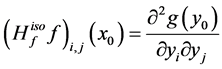 . From the Hessian matrix, we define a
 ![]() - functional of
- functional of  in isometric coordinates, denoted by
![]() , as
, as
 (1.14)
where  is a probability measure on
 ![]() which has strictly positive density everywhere on the interior of
which has strictly positive density everywhere on the interior of
![]() . It is clear that
. It is clear that ![]() of the
of the  component functions of
  are zero as their pullbacks to
 ![]() are linear functions. Indeed,
are linear functions. Indeed, ![]() has a
has a  -dimensional null space, consisting of the span of the constant functions and the d component functions of
 ; see [51] (Corollary 4). The Hessian matrix and the
 ![]() -functional in isometric coordinates introduced above are unfortunately not computable without knowing the isometric coordinate system
-functional in isometric coordinates introduced above are unfortunately not computable without knowing the isometric coordinate system  first. To obtain a functional with the same property but independent of the isometric coordinate system
 , a Hessian matrix and the
 ![]() -functional in local tangent coordinate systems are introduced in [51] . Qiang Ye and Weifeng Zhi [52] developed a discrete version of the Hessian Eigenmaps method of Donoho ad Grims.
-functional in local tangent coordinate systems are introduced in [51] . Qiang Ye and Weifeng Zhi [52] developed a discrete version of the Hessian Eigenmaps method of Donoho ad Grims.
15. Miscellaneous
15.1. Vector Quantization
The main references for vector quantization are [40] and [53] . In [53] it is introduced a hybrid non-linear dimension reduction method based on combining vector quantization for first clustering the data, after constructing the Voronoi cell clusters, applying PCA on them. In [40] both non-linear method i.e., vector quantization and non-linear PCA (using a five layer neural network) on the image data set have been used. It turns out that the vector quantization achieved much better results than non-linear PCA.
15.2. Genetic and Evolutionary Algorithms
These algorithms introduced in [54] are in fact optimization algorithms based on Darwinian theory of evolution which uses natural selection and genetics to find the optimized solution among members of competing population. There are several references for genetic and evolutionary algorithms [55] , see [56] for more detail. An evolutionary algorithm for optimization is different from classical optimization methods in several ways:
• Random Versus Deterministic Operation
• Population Versus Single Best Solution
• Creating New Solutions Through Mutation
• Combining Solutions Through Crossover
• Selecting Solutions Via “Survival of the Fittest”
• Drawbacks of Evolutionary Algorithms In [55] using genetic and evolutionary and algorithms combine with a k-nearest neighbor classifier to reduce the dimension of feature set. Here Input is population matrices which are in fact random transformation matrices , then algorithms will find output
  so that the k-nearest neighbor classifier using the new features
  classifies the training data most accurately.
15.3. Regression
We can use Regression methods for dimension reduction when we are looking for a variable function
 for a given data set variables
 . Under assumption that the
  s are uncorrelated and relevant to expanding the variation in
![]() . Of course in modern data mining applications however such assumptions rarely hold. Hence we need a dimension reduction for such a case. We can list well-known dimension reduction methods as follows:
. Of course in modern data mining applications however such assumptions rarely hold. Hence we need a dimension reduction for such a case. We can list well-known dimension reduction methods as follows:
• The Wrapper method in machine learning community [57]
• Projection pursuit regression [36] [58]
• Generalized linear models [59] [60]
• Adaptive models [61]
• Neural network models and sliced regression and Principal hessian direction [62]
• Dimension reduction for conditional mean in regression [63]
• Principal manifolds and non-linear dimension reduction [64]
• Sliced regression for dimension reduction [65]
• Canonical correlation [66]
Acknowledgements
Our research has received funding from the (European Union) Seventh Framework Programme ([FP7/2007- 2013]) under grant agreement n [314329]. we would like to thank Eu-Commission for the support.
References
- Donoho, D.L. (2000) High-Dimensional Data Analysis: The Curses and Blessings of Dimensionality. Lecture Delivered at the “Mathematical Challenges of the 21st Century” Conference of the American Math. Society, Los Angeles. http://www-stat.stanford.edu/donoho/Lectures/AMS2000/AMS2000.html
- Diamantaras, K.I. and Kung, S.Y. (1996) Principal Component Neural Networks: Theory and Applications. John Wiley, NY.
- Person, K. (1901) On Lines and Planes of Closest Fit to System of Points in Space. Philiosophical Magazine, 2, 559-572. http://dx.doi.org/10.1080/14786440109462720
- Jenkins, O.C. and Mataric, M.J. (2002) Deriving Acion and Behavior Primitives from Human Motion Data. International Conference n Robots and Systems, 3, 2551-2556.
- Jain, A.K. and Dubes, R.C. (1962) Algorithms for Clastering Data. Prentice Hall, Upper Saddle River.
- Mardia, K.V., Kent, J.T. and Bibby, J.M. (1995) Multivariate Analysis Probability and Mathematical Statistics. Academic Press, Waltham.
- (2002) Francesco Camastra Data Dimensionality Estimation Methods, a Survey INFM-DISI, University of Genova, Genova.
- Fukunaga, K. (1982) Intrinsic Dimensionality Extraction, in Classification, Pattern Recognition and Reduction of Dimensionality, Vol. 2 of Handbook of Statistics, North Holland, 347-362.
- Torgerson, W.S. (1952) Multidimenmsional Scaling I: Theory and Methode. Psychometrika, 17, 401-419. http://dx.doi.org/10.1007/BF02288916
- Teng, L., Li, H., Fu, X., Chen, W. and Shen, I-F. (2005) Dimension Reduction of Microarrey Data Based on Local Tangent Space Aligment. Proceedings of the 4th IEEE international Conference on Cogenitive Informatics, 154-159.
- Williams, C.K.I. (2002) On a Connection between Kernel PCA and Metric Multidimensional Scaling. Machine Learning, 46, 11-19. http://dx.doi.org/10.1023/A:1012485807823
- Chatfield, C. and Collins, A.J. (1980) Introduction to Multivariate Analysis. Chapman and Hill. http://dx.doi.org/10.1007/978-1-4899-3184-9
- Platt, J.C. (2005) FastMap, MetricMap, and Landmark MDS are all Nyström algorithms. Proceddings of the 10th International Workshop on Artificial Intelligence and Statistics, 15, 261-268.
- Roweis, S.T. (1997) EM Algorithms for PCA and SPCA. Advances in Neural Information Processing Systems, 10, 626-632.
- Lawrence, N.D. (2005) Probabilistic Non-Linear Proncipal Component Analysis with Gaussian Process Latent Variable Models. Journal of Machine Learning Research, 6, 1783-1816.
- Welling, M., Rosen-Zvi, M. and Hinton, G. (2004) Exponential Family Harmoniums with an Application to Information Retrieval. Advances in Neural Information Processing Systems, 17, 1481-1488.
- Turk, M.A. and Pentland, A.P. (1991) Face Recognition Using Eigenfaces. Proceedings of the Computer Vision and Pattern Recognition 1991, Maui, 586-591. http://dx.doi.org/10.1109/CVPR.1991.139758
- Huber, R., Ramoser, H., Mayer, K., Penz, H. and Rubik, M. (2005) Classification of Coins Using an Eigenspace Approach. Pattern Recognition Letters, 26, 61-75. http://dx.doi.org/10.1016/j.patrec.2004.09.006
- Posadas, A.M., Vidal, F., de Miguel, F., Alguacil, G., Pena, J., Ibanez, J.M. and Morales, J. (1993) Spatialtemporal Analysis of a Seismic Series Using the Principal Components Method. Journal of Geophysical Research, 98, 1923- 1932. http://dx.doi.org/10.1029/92JB02297
- Partridge, M. and Calvo, R. (1997) Fast Dimensionality Reduction and Simple PCA. Intelligent Data Analysis, 2, 292-298.
- Schölkopf, B., Smola, A. and Müller, K.R. (1998) Nonlinear Component Analysis as a Kernel Eigenvalue Problem. Neural Computation, 10, 1299-1319.
- Shawe-Taylor, J. and Christianini, N. (2004) Kernel Methods for Pattern Analysis. Cambridge University Press, Cambridge.
- Tipping, M.E. (2000) Sparse Kernel Principal Component Analysis. Advances in Neural Information Processing Systems, 13, 633-639.
- Kim, K.I., Jung, K. and Kim, H.J. (2002) Face Recognition Using Kernel Principal Component Analysis. IEEE Signal Processing Letters, 9, 40-42. http://dx.doi.org/10.1109/97.991133
- Hoffmann. H. (2007) Kernel PCA for Novelty Detection. Pattern Recognition, 40, 863-874. http://dx.doi.org/10.1016/j.patcog.2006.07.009
- Lima, A., Zen, H. Nankaku, Y. Miyajima, C. Tokuda, K. and Kitamura. T. (2004) On the Use of Kernel PCA for Feature Extraction in Speech Recognition. IEICE Transactions on Information Systems, E87-D, 2802-2811.
- Duda, R.O., Hart, P.E. and Stork, D.G. (2001) Pattern Classification, Wiley Interscience, New York.
- Shin, Y.J. and Park, C.H. (2011) Analysis of Correlation Based Dimension Reduction Methods. International Journal of Applied Mathematics and Computer Science, 21, 549-558.
- Fukunaga, K. (1990) Introduction to Statistical Pattern Recognition. 2nd Edition, Academic Press, San Diego.
- Hotelling, H. (1936) Relations between Two Sets of Vertices. Biometrika, 28, 321-377.
- Sun, Q., Zeng, S., Liu, Y., Heng, P. and Xia, D. (2005) A New Methode of Feature Fusion and Its Application in Image Recognition. Pattern Recognition, 38, 2437-2448. http://dx.doi.org/10.1016/j.patcog.2004.12.013
- Hastie, T. and Stuezle, W. (1989) Principal Curves. Journal of the American Statistical Association, 84, 502-516.
- Kegl, B. and Linder, T. (2000) Learning and Design of Principal Curves. IEEE Transactions on Pattern Analysis and Machine Intelligence, 22, 281-297.
- Ozertem, U. and Erdogmus, D. (2011) Locally Defined Principal Curves and Surfaces. Journal of Machine Learning Research, 12, 1249-1286.
- Malthouse, E. (1996) Some Theoretical Results on Nonlinear Principal Component Analysis. citeseer.nj.net.com/malthouse96some.html
- Carreira-Perpinan, M.A. (1997) A Review of Dimension Reduction Tecniques. Technical Report CS-96-09. Department of Computer Science, University of Sheffield, Sheffield.
- Tibshirani, R. (1992) Principal Curves Revisited. Statistics and Computing, 2,183-190. http://dx.doi.org/10.1007/BF01889678
- Bishop, C.M. (1995) Neural Networks for Pattern Recognition. Oxford University Press, New York.
- Ripley, B.D. (1996) Pattern Recognition and Neural Networks. Cambridge University Press, Cambridge.
- Spierenburg, J.A. (1997) Dimension Reduction of Images Using Neural Networks. Master’s Thesis, Leiden University, Leiden.
- Kramer, M.A. (1991) Non-Linear Principal Component Analysis Using Associative Neural Networks. AIChE Journal, 37, 233-243. http://dx.doi.org/10.1002/aic.690370209
- Press, W.H., Flannery, B.P., Teukolsky, S.A. and Vettering, W.T. (1992) Numerical Recips in C: The Art of Scientific Computing. 2nd Edition, Cambridge University Press, Cambridge.
- Fowlkers, C., Belongie, S., Chung, F. and Malik, J. (2004) Specral Grouping Using the Nysroem Method. IEEE Transactions on Pattern Analysis and Machine Intelligence, 26, 214-225.
- Marida, K.V., Kent, J.T. and Bibby, J.M. (1995) Multivariate Analysis. Probability and Mathematical Statistics. Academic Press, Waltham.
- Faloutsos, C. and Lin, K.I. (1995) FastMap: A Fast Algorithm for Indexing, Data-Mining and Visualization of Traditional and Multimedia Datasets. In: Carey, M.J. and Schneider, D.A., Eds., Proceedings of the 1995 ACM SIGMOD International Conference on Management of Data, San Jose, 163-174. http://dx.doi.org/10.1145/223784.223812
- Fodor, I.K. (2002) A Survey of Dimension Reduction Techniques. Center for Applied Scientific Computing, Livermore National Laborary, Livermore.
- Chung, F.R.K. (1997) Spectral Graph Theory. American Mathematical Society. CBMS Regional Conference Series in Mathematics in American Mathematical Society, 212, 92.
- Belkin, M. and Niyogi, P. (2003) Laplacian Eigenmaps for Dimensionality Reduction and Data Representation. Neural Computation, 15, 1373-1396. http://dx.doi.org/10.1162/089976603321780317
- Rivest, R., Cormen, T., Leiserson, C. and Stein, C. (2001) Introduction to Algorithms. MIT Press, Cambridge.
- Kumar, V., Grama, A., Gupta, A. and Karypis, G. (1994) Introduction to Parallel Computing. Benjamin-Cummings, Redwood City.
- Donoho, D. and Grimes, C. Hessian Eigenmaps: Locally Linear Embedding Techniques for High-Dimensional Data. Proceedings of National Academy of Sciences, 100.
- Ye, Q. and Zhi, W.F. (2003) Discrete Hessian Eigenmaps Method for Dimensionality Reduction.
- Kamhaltla, N. and Leen, T.K. (1994) Fast Non-Linear Dimension Reduction. In: Advances in Neural Information Processing Systems, Morgan Kaufmann Publishers, Inc., Burlington, 152-159.
- Goldberg, D.E. (1989) Genetic Algorithms in Search, Optimization and Machin Learning. Addisn Wesley, Reading.
- Raymer, M.L., Goodman, E.D., Kuhn, L.A. and Jain, A.K. (2000) Dimensionality Reduction Using Genetic Algorithms. IEEE Transactions on Evolutionary Computation, 4, 164-171. http://dx.doi.org/10.1109/4235.850656
- Jones, G. (2002) Published Online: 15 APR. University of Sheffield, Sheffield.
- Kohavi, R. and John, G. (1998) The Wrapper Approach. In: Liu, H. and Motoda, H., Eds., Feature Extraction, Construction and Selection: A Data Mining Perspective, Springer Verlag, Berlin, 33-50. http://dx.doi.org/10.1007/978-1-4615-5725-8_3
- Huber, P.J. (1985) Projection Persuit. Annals of Statistics, 13, 435-475. http://dx.doi.org/10.1214/aos/1176349519
- McCullagh, P. and Nelder, J.A. (1989) Generalized Linear Models. Chapman and Hall, Boca Raton. http://dx.doi.org/10.1007/978-1-4899-3242-6
- Dobson, A.J. (1990) An Introduction to Generalized Linear Models. Chapman and Hall, London. http://dx.doi.org/10.1007/978-1-4899-7252-1
- Leathwick, J.R. Elith, J. and Hastie, T. (2006) Comparative Performance of Generalized Additive Models and Multivariate Adaptive Regression Splines for Statistical Modelling of Species Distributions. Ecological Modelling, 188-196. http://www.stanford.edu/~hastie/Papers/Ecology/leathwick_etal_2006_mars_ecolmod.pdf
- Li, K.C. (2000) High Dimensional Data Analysis via SIR/PHD Approach. Lecture Note in Progress. http://www.stat.ucla.edu/kcli/
- Dennis Cook, R. and Li, B. (2002) Dimension Reduction for Conditional Mean in Regression. Annals of Statistics, 30, 455-474. http://dx.doi.org/10.1214/aos/1021379861
- Zhang, Z. and Zha, H. (2002) Principal Manifolds and Nonlinear Dimension Reduction via Local Tangent Space Alignment. http://arxiv.org/pdf/cs.LG/0212008.pdf
- Wang, H. and Xia, Y. (2008) Sliced Regression for Dimension Reduction. Peking University & National University of Singapore, Journal of the American Statistical Association, 103, 811-821.
- Feng, W.K., He, X. and Shi, P. (2002) Dimension Reduction Based on Canonical Correlation. Statistica Sinica, 12, 1093-1113.
- Lectures on Fractals and Dimension Theory. http://homepages.warwick.ac.uk/masdbl/dimensiontotal.pdf
Appendix. Fractal and Topological Dimension
The main Reference for this appendix is [67]. Local (or topological) Methods (1): The definition of topological dimension was given by Brouwer in 1913: A. Heyting, H. Freudenthal, Collected Works of L.E.J Brouwer, North Holland Elsevier, 1975.
To begin at the very beginning: How can we best define the dimension of a closed bounded set , say?
• When ![]() is a manifold then the value of the dimension is an integer which coincides with the usual notion of dimension;
is a manifold then the value of the dimension is an integer which coincides with the usual notion of dimension;
• For more general sets ![]() we can have fractional dimensional
we can have fractional dimensional
• Points, and countable unions of points, have zero dimension.
Local (or topological) Methods (2): The earliest attempt to define the dimension:
Definition 1 We can define the Topological dimension  by induction. We say that
 ![]() has zero dimension if for every point
has zero dimension if for every point ![]() every sufficiently small ball about
every sufficiently small ball about  has boundary not intersecting
![]() . We say that
. We say that ![]() has dimension
has dimension  if for every point
 ![]() every sufficiently small ball about
every sufficiently small ball about  has boundary intersecting
 ![]() in a set of dimension
in a set of dimension .
.
Local (or topological) Methods (3):
Definition 2 Given![]() , let
, let  be the smallest number of
  -balls needed to cover
![]() . The Box dimension is
. The Box dimension is

Example 1 For 

Local (or topological) Methods (4): The Hausdorff dimension  for a closed bounded set
  is defined as follows:
Definition 3 Consider a cover  for
for ![]() by open sets. For
by open sets. For ![]() we can define
we can define

where the infimum is taken over all open covers  such that
 .Then
.Then
![]() and finally•
and finally• 
• Fact1: For any countable set ![]() we have
we have 
• Fact2: 
Local (or topological) Methods (4) as shown in Figure 1.
Local (or to pological) Methods (5):
Example 2 (von Koch curve: [ ] The von Koch curve is a standard fractal construction. Starting from
 , we associate to each piecewise linear curve
  in the plane ( which is a union of
 ![]() segments of length
segments of length ) a new one
 .This is done by replacing the middle third of each line segment by the other two sides of an equilateral triangle bases there. Alternatively, one can start from an equilateral triangle and apply this iterative procedure to each of the sides one gets a snowflake curve.
For ![]() = von Koch curve, both the box dimension and Hausdorff dimension are equal in fact, as shown in Figure 2:
= von Koch curve, both the box dimension and Hausdorff dimension are equal in fact, as shown in Figure 2:

Example 3 (![]() : the Middle third Cantor set
: the Middle third Cantor set ,
,  This is the set of closed set of points in the unit interval whose triadic expansion does not contain any occurrence of the digit
 :
:

For the middle third Cantor set both the Box dimension and the Hausdorf dimension are 
The set  is the set of points whose continued fraction expansion contains only the terms
  and
and . Unlike the Middle third Cantor set, the dimension of this set is not explicitly known in a closed form and can only be numerically estimated to the desired level of accuracy. as shown in Figure 3, For the Sierpinski carpet both the Box dimension and the Hausdorff dimension are equal to
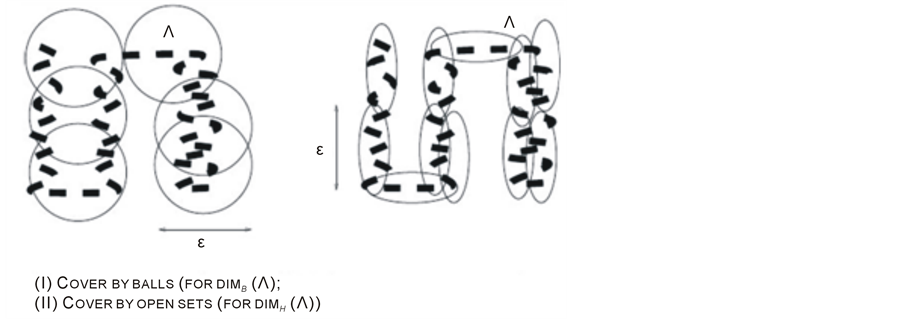
Figure 1. (I) Cocer by balls, (II) Cover by open sets.
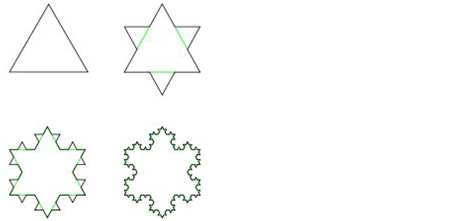
Figure 2. The construction of von Koch-curve.
Figure 3. The construction Sierpinski Carpet.sp;