American Journal of Operations Research
Vol. 2 No. 2 (2012) , Article ID: 19928 , 10 pages DOI:10.4236/ajor.2012.22018
A Construction Heuristic for the Split Delivery Vehicle Routing Problem
1Industrial and Information Engineering Department, University of Tennessee, Knoxville, USA
2Industrial and Manufacturing Engineering Department, Pennsylvania State University, University Park, USA
Email: jwilck@utk.edu, tmc7@psu.edu
Received February 18, 2012; revised March 17, 2012; accepted March 29, 2012
Keywords: Vehicle Routing Problem; Transportation; Construction Heuristics
ABSTRACT
The Split Delivery Vehicle Routing Problem (SDVRP) is a relaxation of the Capacitated Vehicle Routing Problem (CVRP) where customers may be assigned to multiple routes. A new construction heuristic is developed for the SDVRP and computational results are given for thirty-two data sets from previous literature. With respect to the total travel distance, the construction heuristic compares favorably versus a column generation method and a two-phase method. In addition, the construction heuristic is computationally faster than both previous methods. This construction heuristic could be useful in developing initial solutions, very quickly, for a heuristic, algorithm, or exact procedure.
1. Introduction
The Vehicle Routing Problem (VRP) is a prominent combinatorial optimization problem in distribution planning. Various forms of the VRP are studied for both theoretical and practical purposes. The solution quality of these problems is essential to the logistics industry when considering transportation costs. Dantzig and Ramser [1] first exhibited these cost savings by providing a formulation and solution approach for gasoline distribution. Toth and Vigo [2] estimate that computer-generated solutions for distribution problems reduce transportation costs by 5% - 20%, and this is a significant decrease since transportation costs represent between 10% - 20% of the final cost of a unit. Review literature for the VRP includes a survey by Toth and Vigo [3] for exact solution procedures, whereas Cordeau et al. [4-5] survey heuristic procedures.
A well-studied form of the VRP is the Capacitated Vehicle Routing Problem (CVRP). The CVRP establishes routes to a set of customers from a single depot to minimize the total distance traveled. The problem is constrained by the vehicle capacity while meeting customer demand. By definition, a customer is on exactly one route. The Split Delivery Vehicle Routing Problem (SDVRP) is a relaxation of the CVRP. The SDVRP allows customers to be serviced by more than one vehicle route, which usually reduces the number of routes and the total distance traveled [6]. Generally, the SDVRP takes more computer time to solve than the CVRP since the feasible space is larger [6-8]. In this paper a set of feasible solutions is generated for the SDVRP using a construction heuristic, and the solution with the shortest travel distance is outputted. Recent literature surveys of the SDVRP include [9-11].
The SDVRP is appropriate for many CVRP applications where customers can be visited more than once. Numerous applications for the CVRP are noted in the literature [3,12], with the primary emphasis being the distribution of various goods. Dror and Trudeau [6,7] formally introduced the SDVRP. The primary motivation to split a customer’s demand over multiple routes is to reduce the travel distance and the number of vehicle routes. If each vehicle has the same capacity, then the minimum number of routes is the total demand divided by the vehicle capacity rounded up to the nearest integer.
Dror and Trudeau [6,7] proved, given that the distance between nodes follows the triangle inequality, there exists an optimal solution where no two routes can have more than one split demand point in common, and that there exists an optimal solution with no k-split cycles (for any k). Based on these proofs, Dror and Trudeau [7] devised a heuristic to solve the SDVRP given an initial CVRP solution by splitting the demand of a node to fill the routes to capacity. This algorithm allows for additional routes over the minimum number of routes. The heuristic does not eliminate k-split cycles; however, no 2-split or 3-split cycles were observed in any of the resulting solutions.
Dror et al. [8] extended the formulation of Dror and Trudeau [6,7] with additional constraints, and developed a constraint relaxation branch and bound algorithm. The directed arc formulation allows the number of vehicle routes to vary from the minimum number to the number of customers. The additional constraints strengthen the subtour elimination constraints, eliminate some fractional cycles when the binary decision variables are relaxed, and impose an upper bound on the number of arcs used in an optimal solution. Results of the algorithm were given for problems with 10, 15, and 20 customers and optimality gaps were reported. The optimality gap was within 10% for 10 customer problems, 20% for 15 customer problems, and 30% for 20 customer problems. However, in order to reduce the number of constraints produced, arcs over a certain length were eliminated from consideration.
The results from [6-8] show that the percent reduction in travel distance, when compared to the CVRP, is most prominent among problems where customers have high demands (i.e., more than 10% of the vehicle capacity). The results also indicate that good solutions to the SDVRP tend to have routes that sweep geographic areas, and that customers with split demand over multiple routes usually have above average demand. The results showed that the SDVRP solution used fewer routes than the CVRP solution; however, the SDVRP solution did not always use the minimum number of routes. The computer time to obtain the SDVRP solution was longer than the time to compute the CVRP solution.
Frizzell and Giffin [13,14] solved the SDVRP on grid networks in their first paper and with time windows on grid networks in their second paper. Archetti et al. [15] developed a tabu search algorithm for the SDVRP. Archetti et al. [16] analyzed the worst-case properties of the SDVRP, where they show that the savings are at most 50% over the optimal CVRP solution. Archetti et al. [17] discussed when demand splitting is most beneficial. Their results indicated that demand splitting is best when the mean customer demand is just over half of the vehicle capacity and when customer demand variance is low. Lee et al. [18] developed a dynamic programming model for the vehicle routing problem with split pick-ups with an uncountable (infinite) number of state and action spaces.
Belenguer et al. [19] performed a polyhedral study on the SDVRP to produce lower bounds through formulating the problem with undirected arcs by assuming symmetric distances. Using a cutting-plane algorithm in conjunction with a relaxed formulation, they were able to obtain feasibility gaps within 12% for problems with 50, 75, and 100 customers. They did not report computation time, only the number of iterations and the number of cuts.
Jin et al. [20] developed a two-stage algorithm to solve the SDVRP using valid inequalities. Jin et al. [21] presented a column generation procedure that provides comparable lower and upper bounds for the data sets developed by [19]. Jin et al. [21] allowed for additional routes above the minimum number of vehicle routes. Chen et al. [22] presented a mixed integer program and a variable length record-to-record travel algorithm. They also provided computational results for existing and new data sets. References [9,22,23] used the Clarke-Wright Algorithm [24] for the CVRP to provide an initial starting solution for the SDVRP. Burrows [25] showed that the SDVRP could be modified by splitting customer demand into smaller quantities on the same node, and then solved using CVRP methods. Recent theses addressing the SDVRP, or close variants, include [23,26-29].
Direct applications of the SDVRP have been noted in literature. Mullaseril et al. [30] modeled a cattle feed distribution problem as an SDVRP with time windows. They developed a solution algorithm that uses k-split interchanges and route addition. Sierksma and Tijssen [31] model a helicopter crew-scheduling problem using an SDVRP model, and they developed two solution approaches. The first used a relaxed linear program and column generation scheme to find a solution. The second used a cluster-and-route procedure. Song et al. [32] modeled a newspaper distribution process as a SDVRP and solved using a two-phase procedure. The first phase allocates customers using a binary program and the second phase generates vehicle routes.
This paper presents a construction heuristic that generates a set of feasible solutions for the SDVRP, and the solution with the shortest travel distance is outputted. This construction heuristic is compared against two previous methods using 32 data sets from earlier literature. The solutions from this construction heuristic could then be used for other heuristics, algorithms, or exact methods. The remainder of this paper is organized as follows. The next section provides a mathematical formulation of the SDVRP. This is followed by the SDVRP construction heuristic, computational experience, and concluding remarks.
2. SDVRP Formulation
The SDVRP can be defined as follows. Let G = (N, A) be a complete and directed graph, where N = {1, 2, ···, n} is the set of nodes and A = {(i, j), i, j  N, i ¹ j} is the set of arcs. Node 1 represents the depot and nodes {2, 3, ···, n} represent customers. The cost of traversing an arc is denoted by cij, and it is assumed that cij is non-negative and the triangle inequality holds. The demand of each customer is denoted by di. The vehicles, assumed to be identical, have a capacity of Q and are based at the depot. The total demand D, and vehicle capacity are used to determine the minimum number of routes K. The SDVRP consists of determining K routes from the depot by minimizing the total distance traveled, while satisfying the customer demand and not exceeding vehicle capacity.
The following formulation is a combination of the directed graph formulation [19] and the undirected graph formulation [8]. This formulation assumes that cij satisfies the triangle inequality and that exactly the minimum number of vehicle routes, K, is used. The formulation does not assume that distances are symmetric.
Indexed Sets:
i = {1, 2, ···, n}; node index j = {1, 2, ···, n}; node index k = {1, 2, ···, m}; route index Parameters:
m: the number of vehicle routes n: the number of nodes Q: the vehicle capacity cij: the cost or distance from node i to node j di: the demand of customer i (where d1 = 0)
Decision Variables:
xijk: 1 when arc (i, j) is traversed on route k; 0 otherwise uik: free variable used in the subtour elimination constraints yik: 1 when node i is visited on route k; 0 otherwise vik: a variable that denotes the amount of material delivered to node i on route k Without loss of generality, yik and vik are not defined for i = 1.
Objective:
Minimize
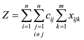 (1)
(1)
Constraints:
 (2)
(2)
 (3)
(3)
 (4)
(4)
 (5)
(5)
 (6)
(6)
 (7)
(7)
 (8)
(8)
 (9)
(9)
 (10)
(10)
 (11)
(11)
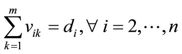
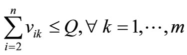
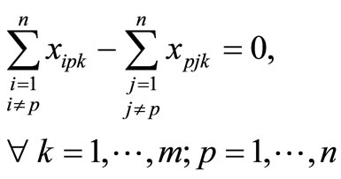
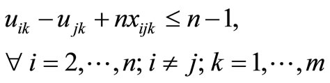
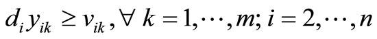
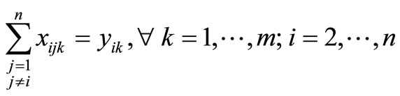
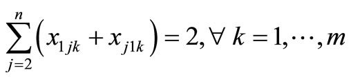
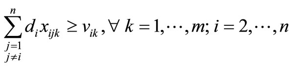
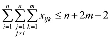
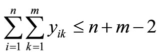
The objective is represented by (1), which is to minimize the total distance traveled. Constraints (2) and (3) guarantee that all customer demand is satisfied without violating vehicle capacity. Constraints (4) and (5) ensure flow conservation and that subtours are eliminated, respectively. Constraints (6) and (7) force the binary variables to be positive if material is delivered to node i on route k. Constraint (8) ensures that the depot is entered and exited on every vehicle route, and Constraints (9)- (11) provide variable restrictions. Additional, mathematically redundant, constraints that can be used to possibly strengthen the formulation are:
 (12)
(12)
 (13)
(13)
 (14)
(14)
 (15)
(15)
 (16)
(16)
 (17)
(17)
 (18)
(18)
 (19)
(19)
 (20)
(20)
 (21)
(21)
 (22)
(22)
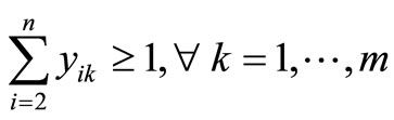
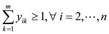
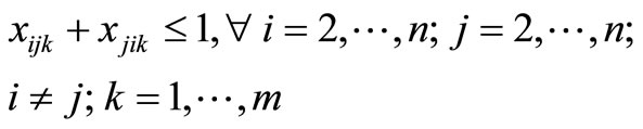
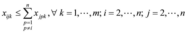
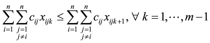
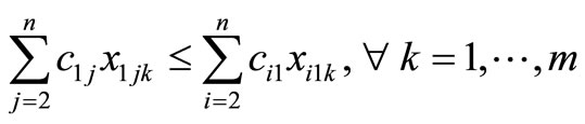
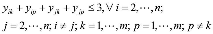
Constraint (12) guarantees that if a customer is visited then material is delivered, and Constraint (13) does not allow material to be delivered unless a customer is visited. First introduced by Belenguer et al. [19], Constraints (14) and (15) ensure each route is used and a customer is visited at least once, respectfully. Constraint (16) eliminates two-node subtours. Dror et al. [8] introduced constraint (17), which eliminates some k-split cycles by placing an upper-bound on the number of arcs that can be used in an optimal solution. Constraint (18), which follows from constraint (17), restricts the total number of customer visits within an optimal solution. Constraint (19), introduced by Dror et al. [8], removes some types of fractional cycles when the binary restrictions of xijk are relaxed. Constraint (20) eliminates alternative optimal solutions for routes by sorting the routes from shortest to longest. Alternative optimal solutions are nullified by Constraint (21) for the direction of the particular route by having the shortest arc traversed first of the two arcs adjacent to the depot. Split deliveries are forbidden by Constraint (22) to nodes i and j on both routes k and p. There exist additional constraints that were not listed; however, only constraints that were beneficial in preliminary testing were noted.
3. SDVRP Construction Heuristic
The heuristic procedure presented in this section constructs a set of feasible solutions to the SDVRP. The first procedure of the heuristic initializes the input. The second procedure assigns customers to vehicle routes, iteratively. The order of each route is then determined by a traveling salesman problem (TSP) solution procedure, finalizing the solution. Finally, the solution is outputted. The computer code for the heuristic assumes that customer demand and vehicle capacity are integers. Similar to the flow formulation in Section 2, the computer code for the heuristic does not assume symmetric distances between two nodes. Ties are broken arbitrarily, unless otherwise specified.
3.1. Partition Procedure
The partition procedure assigns customers and their demand to vehicle routes. Initially, the procedure checks for feasibility (i.e., adequate capacity). The iterative process begins with Control 1, which is completed for each vehicle route. A customer, with unsatisfied demand, is selected and assigned to the vehicle route in Control 1. The capacity threshold is calculated in Control 2. If the vehicle is not loaded within the capacity threshold, then the algorithm proceeds to Control 3. Otherwise, Control 1 is repeated for the next vehicle route. Control 3 selects a number of customers closest to the set of customers already assigned to the vehicle route and determines whether or not they will be added to the route. Control 3 is repeated until the vehicle is loaded within the capacity threshold or until all customer demand is satisfied. The outputs from this procedure are the vik and yik variables. This procedure is shown in Figure 1.
There are three decisions made in the partition procedure for each vehicle route, each decision corresponds to a control from Figure 1. Control 1 selects an initial node
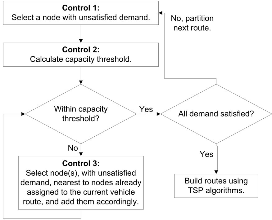
Figure 1. Partition procedure for SDVRP construction heuristic.
to begin the vehicle route. Control 2 calculates the capacity threshold. Control 3 determines how many nodes to evaluate per iteration. This dissertation will focus on eight rules for Control 1 and three rules each for Control 2 and Control 3; thus, there are seventy-two possible combinations if every rule is completed for the three controls. There are an infinite amount of rules for each Control, but based on preliminary testing, intuition, and time constraints we have focused on a smaller set of rules.
Control 1: The initial node for each vehicle route is selected from the set of customers with unsatisfied demand. This initial node is selected using one of the following eight rules: furthest node from the depot, closest node from the depot, median node with respect to distance from depot, node with highest demand, node with smallest demand, furthest node on smallest arc (i.e., the arc (i,j), where i ≠ j, i ≠ 1, j ≠ 1, for which cij is the smallest), random node, and furthest node based on the arc from the Clarke-Wright [24] procedure. The ClarkeWright procedure calculates a savings sij = c1i – cij + cj1 for each arc (i,j) where i ≠ j, i ≠ 1, j ≠ 1, and the arc with the largest savings is selected. These eight rules may select the same initial node for a particular vehicle route; however, they have the potential to be diverse in their selection.
Control 2: The capacity threshold allows the spare vehicle capacity (i.e., the total amount of spare vehicle capacity across all routes, calculated by mQ – D) to be shared amongst all of the vehicle routes. This threshold is calculated by three different rules. The first rule takes the average spare capacity (i.e., remaining spare vehicle capacity divided by the remaining number of vehicle routes), based on the remaining number of vehicle routes, and rounds the answer down to the nearest integer. The second rule takes the average spare capacity, based on the remaining number of vehicle routes, and rounds the answer up to the nearest integer. The third rule allows for the current vehicle route to use all of the spare capacity. These rules can be ignored if there is no spare vehicle capacity, since in that case all of the vehicles must be filled to capacity.
Control 3: The node selection decision evaluates the closest (relative to the nodes already on the vehicle route) one, two, or three nodes per iteration. If only one node is selected, then it is evaluated to determine if all or part of its remaining demand will be placed on the route. All of the demand will be placed on the route if it fits; otherwise, the vehicle route will be filled and the node’s demand will be adjusted. If two nodes are selected, then they are evaluated to determine if one or both can be placed on the vehicle route. Both nodes are added to the route if all of their remaining demand fits on the route. If, individually, both of the nodes remaining demand exceed the vehicle capacity, then only a portion of the closest node’s demand is placed on the route. Otherwise, all of the closest node’s demand is placed on the route and only a portion of the second closest node’s demand. If three nodes are selected, then they are evaluated to determine if one, two, or all will be added to the vehicle route.
The following procedure is an example of one of the 72 combinations. Control 1 takes the furthest node from the depot, Control 2 rounds the average spare capacity up to the nearest integer, and Control 3 evaluates the closest two nodes. This example is shown in Figure 2. In addition to the formulation from Section 2, the following data and variables are used in this procedure:
S: total available spare capacity across all vehicle routes A: average spare capacity per route (i.e., A = S/m, rounded up to the nearest integer)
R: set of nodes with unsatisfied demand Pk: set of nodes currently assigned to route k fi: amount of unsatisfied demand remaining for node i bk: remaining capacity of vehicle k Step 0: Commentary: Step 0 initializes the data and variables for the procedure. Determine constants m, n, D, Q, K, and S. Compute the initial value of A. If m < K, where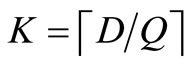 , then STOP the problem is infeasible. Place all nodes in set R, except node 1, which corresponds to the depot. Ensure Pk is empty for all k. Set fi = di for all i. Set
 .
.
Step 1: Commentary: Step 1 selects the furthest node from the depot and adds it to the route currently being constructed, this is the first node added to the route. If , then STOP. From set R, find the node furthest from the depot, call it node i. Place node i in set Pk. If fi > Q, then set yik = 1, vik = Q, fi = fi – Q,
  , and k = k + 1; and go to Step 1. Otherwise, if Q – fi ≤ A, then remove i from set R and set yik = 1, vik = fi,
  ,
,  , fi = 0, and k = k + 1; and go to Step 1. Otherwise, remove i from set R and set yik = 1, vik = fi, bk = Q – fi, and fi = 0; and go to Step 2.
Step 2: Commentary: Step 2 selects nodes to add to the route currently being constructed. If set R is empty, then STOP. If there is only one node in set R, then call it i and go to Step 2f. Otherwise, from set R, find the two closest nodes to the nodes in set Pk. Call the closest node i and the next closest node j.
If fi > bk and fj ≤ bk, then go to Step 2a.
If fi ≤ bk and fj > bk, then go to Step 2b.
If fi ≤ bk, fj ≤ bk, and fi + fj > bk, then go to Step 2c.
If fi ≤ bk, fj ≤ bk, and fi + fj ≤ bk, then go to Step 2d.
If fi > bk and fj > bk, then go to Step 2e.
Step 2a: Commentary: Step 2a adds node j to the route currently being constructed, and then determines if more nodes need to be considered. If bk – fj ≤ A, then remove j from set R, place j in Pk, and set yjk = 1, vjk = fj,  ,
,  , fj = 0, and k = k + 1; and go to Step 1. Otherwise, remove j from set R, place j in Pk, and set yjk = 1, vjk = fj, bk = bk – fj, and fj = 0; and go to Step 2.
Step 2b: Commentary: Step 2b adds node i to the route currently being constructed, and then determines if more nodes need to be considered. If bk – fi ≤ A, then remove i from set R, place i in Pk, and set yik = 1, vik = fi,  ,
,  , fi = 0, and k = k + 1; and go to Step 1. Otherwise, remove i from set R, place i in Pk, and set yik = 1, vik = fi, bk = bk – fi, and fi = 0; and go to Step 2.
Step 2c: Commentary: Step 2c adds node i to the route currently being constructed, and then determines if more nodes need to be considered. If fi = bk, then remove i from set R, place i in Pk, and set yik = 1, vik = fi,  , fi = 0, and k = k + 1; and go to Step 1. Otherwise, remove i from set R, place i in Pk, and set yik = 1, yjk = 1, vik = fi, vjk = bk – fi,
  , fi = 0, fj = fj – vjk, and
 ; and go to Step 1.
Step 2d: Commentary: Step 2d adds nodes i and j to the route currently being constructed, and then determines if more nodes need to be considered. If bk – fi – fj ≤ A, then remove i and j from set R, place i and j in Pk, and set yik = 1,  , vik = fi, vjk = fj, S = S – (bk – fi – fj),
  , fi = 0, fj = 0, and k = k + 1; and go to Step 1. Otherwise, remove i and j from set R, place i and j in Pk, and set yik = 1, yjk = 1,
  , vjk = fj, bk = bk – fi – fj, fi = 0, and fj = 0; and go to Step 2.
Step 2e: Commentary: Step 2e adds node i to the route currently being constructed, and then determines if more nodes need to be considered. Place i in Pk and set yik = 1, vik = bk, fi = fi – bk,  , and k = k + 1; and go to Step 1.
Step 2f: Commentary: Step 2f adds node i to the route currently being constructed. Place i in Pk. If fi ≤ bk, then remove i from set R and set yik = 1, vik = fi, and STOP. Otherwise, set yik = 1, vik = bk, fi = fi – bk,  , and k = k + 1; and go to Step 1.
The above example is the procedure for Control 1 taking the furthest node from the depot, Control 2 rounding the average spare capacity up to the nearest integer, and Control 3 evaluating the closest two nodes. A flowchart of this example is shown in Figure 2. A simple explanation of the steps is as follows. Step 0 is initializes the problem and iteration procedure. Step 1 selects the furthest node and calculates the average spare capacity, performing Control 1 and Control 3. Step 2 selects a node or nodes to add to the vehicle route, performing Control 2. Included within each step are stopping and iterating instructions.
3.2. TSP Solution Procedure
The procedure presented in Section 3.1 assigns customers and their demand to vehicle routes. The order of each individual route is then calculated using a TSP solution procedure. If the number of customers on a particular route is small (i.e., ≤10), then an enumeration method ensures the best possible route with little computation. Initial solution procedures and three-opt neighborhood search procedures can be used for a larger number of customers. Syslo et al. [33] provide detailed algorithms for the TSP, including a branch-and-bound enumeration procedure, a furthest node insertion method, and a threeopt procedure. The outputs from the TSP solution procedure are xijk variables and the objective value. After the
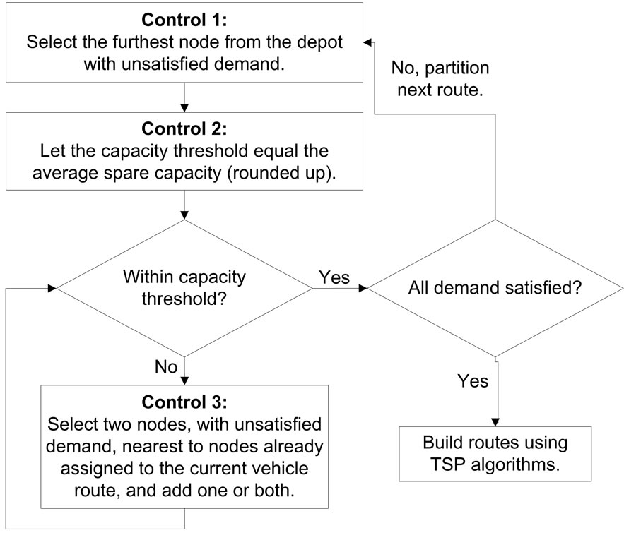
Figure 2. Partition procedure for SDVRP Construction Heuristic where Control 1 takes the furthest node from the depot, Control 2 rounds the average spare capacity up to the nearest integer, and Control 3 evaluates the closest two nodes.
conclusion of the assignment and TSP procedures, an initial feasible solution for the SDVRP is complete.
4. Computational Experience of SDVRP Construction
Initial feasible solutions were constructed for the data sets from Belenguer et al. [19] and Chen et al. [22] based on the Construction Heuristic Procedure described in Section 3.2. The procedure was coded in FORTRAN 95 and compiled by GNU FORTRAN on an Intel Xeon Processor 2.49 GHz computer with 8 GB RAM. The best solution from the 72 combinations was outputted as the final solution for the construction heuristic for each data set. Of the 72 combinations, only nine combinations were needed to find the best solution for all data sets, and those nine combinations come from an initial set of 36 rule combinations. The best nine combinations are listed in Table 1, these combinations result in the best solution for all data sets. For the computational results, the 72 combination runtime, 36 combination runtime, and the best nine runtime are reported.
The number of customers and vehicles for 11 data sets from Belenguer et al. [19] are shown in Table 2. The
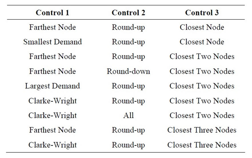
Table 1. Best nine combinations that result in the best solutions for all data sets.
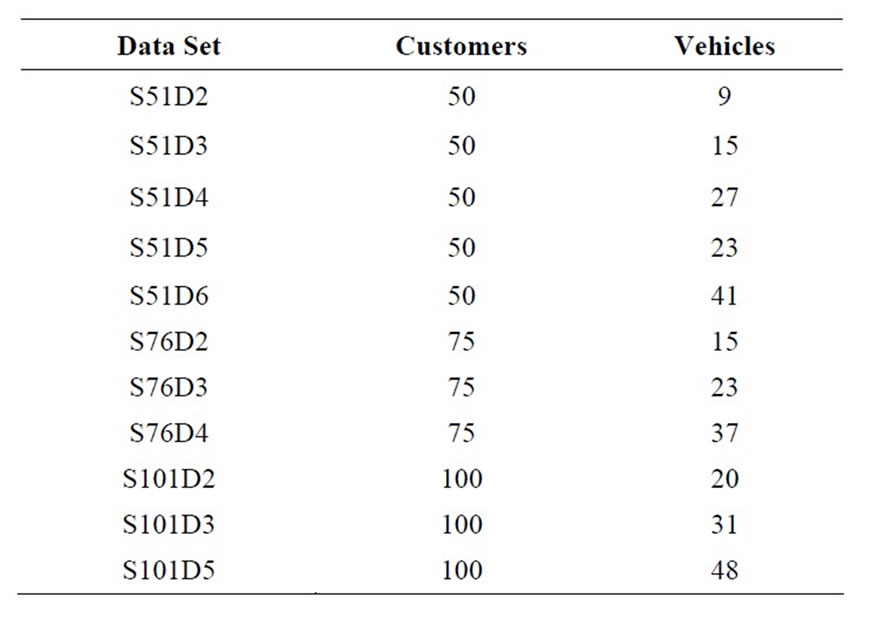
Table 2. Eleven data sets from Belenguer et al. [19].
number of customers ranged from 50 to 100, with an additional node for the depot. The data sets also differ by amount of spare capacity per vehicle. The customers were placed randomly around a central depot and demand was generated randomly based on a high and low threshold.
The number of customers and vehicles for 11 data sets from Belenguer et al. [19] are shown in Table 2. The number of customers ranged from 50 to 100, with an additional node for the depot. The data sets also differ by amount of spare capacity per vehicle. The customers were placed randomly around a central depot and demand was generated randomly based on a high and low threshold. The number of customers and vehicles for 21 data sets from Chen et al. [22] are shown in Table 3. The number of customers ranged from eight to 288, with an additional node for the depot. The data sets do not have any spare vehicle capacity. The customers were placed on rings surrounding a central depot and the demand was either 60 or 90, with a vehicle capacity of 100. Results from Jin et al. [21] and Chen et al. [22] were used as a comparison to the results from the Construction Heuristic Procedure (Section 3) for these 32 data sets, as shown in Tables 4-6.
Comparative results for 11 data sets from Belenguer et al. [19] are shown in Table 4. The construction heuristic produced a solution in the least amount of computer time for each data set (bold), and produced the solution with the least amount of travel distance in four cases (bold). Jin et al. [21] found a better solution for three data sets (bold) and Chen et al. [22] in four cases (bold). However, Jin et al. [21] allowed for additional vehicles in their solution, above the minimum number required for the SDVRP, which increases the cost of the overall system.
Comparative results for 21 data sets from Chen et al. [22] are shown in Table 5. The construction heuristic produced a solution in the least amount of computer time for each data set (bold), and produced the solution with the least amount of travel distance in 16 cases (bold). Chen et al. [22] found a better feasible solution for four data sets (bold). Both methods found a solution with the same objective for data set S1. Chen et al. [22] reported pseudo lower bounds based on a graphical estimation described in Chen [23]. Chen et al. [22] finds a feasible solution that matches this pseudo lower bound for four instances (italic). The construction heuristic finds a feasible solution that matches this pseudo lower bound for five data sets (italic), and finds a feasible solution lower than this bound for nine data sets (italic and underline).
Using lower bounds from previous literature [19,21] the duality gap of the construction heuristic solution is shown in Table 6 for 11 data sets. The duality gap varies from 5.26% to 8.72%, with a solution time of no more than 11.250 seconds. The problem size ranged from 50 to
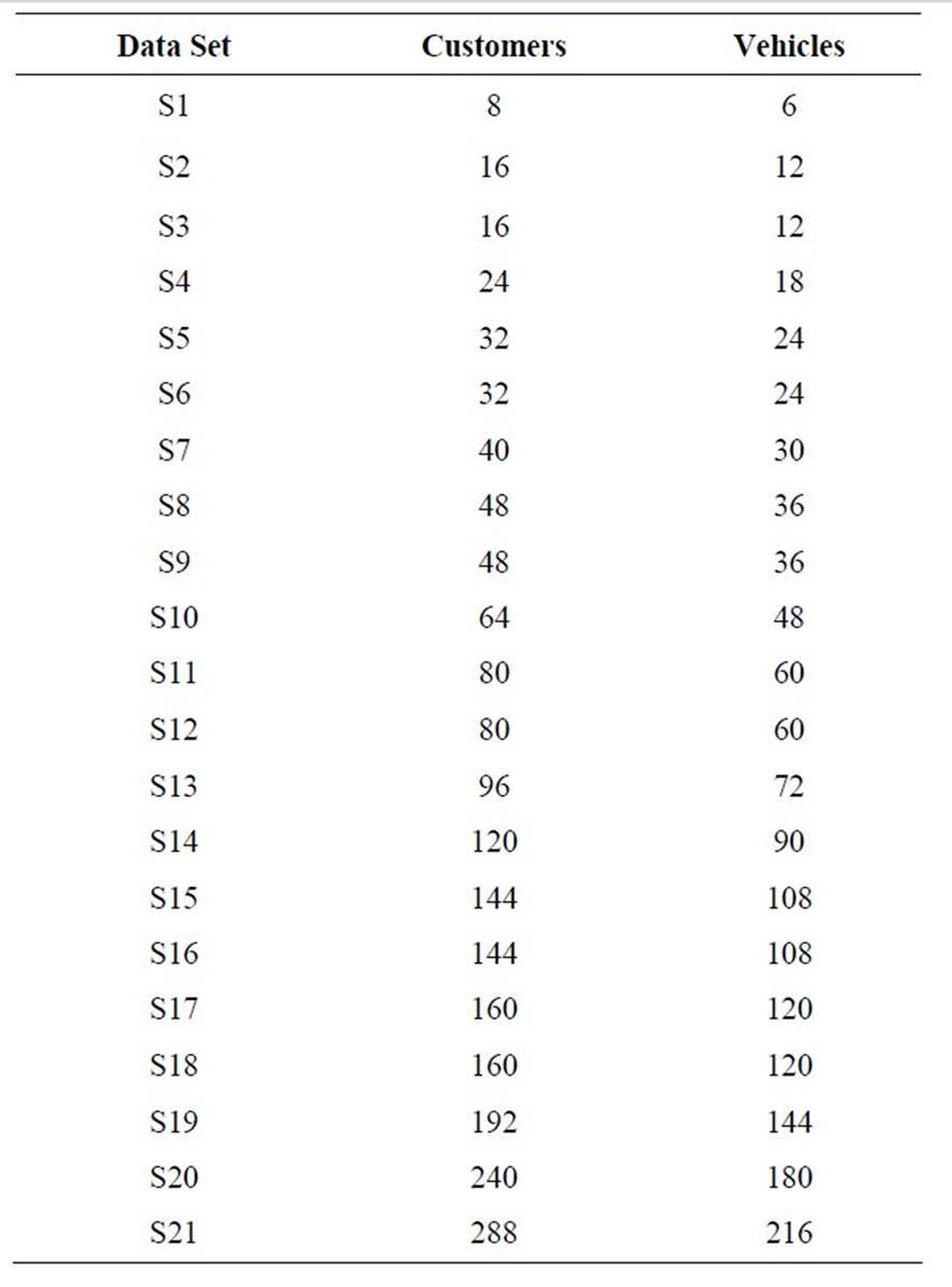
Table 3. Twenty-one data sets from Chen et al. [22].
100 customers and 9 to 48 vehicle routes, as shown in Table 2. Similar results for the 21 data sets are not available since a valid lower bound is not available from previous literature.
The solutions from the construction heuristic are not guaranteed to be local optimal solutions. A neighborhood search was implemented using two or three exchanges amongst the vehicle routes from the best solution and resolving the necessary TSPs. However, the objective value for the 32 data sets only decreased in a few cases, and then only by a small percentage, while using considerable extra computation time (i.e., much longer than the construction heuristic). Therefore, using a neighborhood search was determined to be ineffective.
5. Conclusion
This paper focused on formulating and solving the SDVRP using a flow formulation and a construction heuristic. The primary research result of this paper is a construction heuristic that provides good initial starting solutions (within 8.72% duality GAP for 11 data sets) for the SDVRP in little computer time (within 11.250 seconds for all test cases). The best solution from this construction heuristic could then be used as a starting solution for other methods, such as Tabu search [15], column
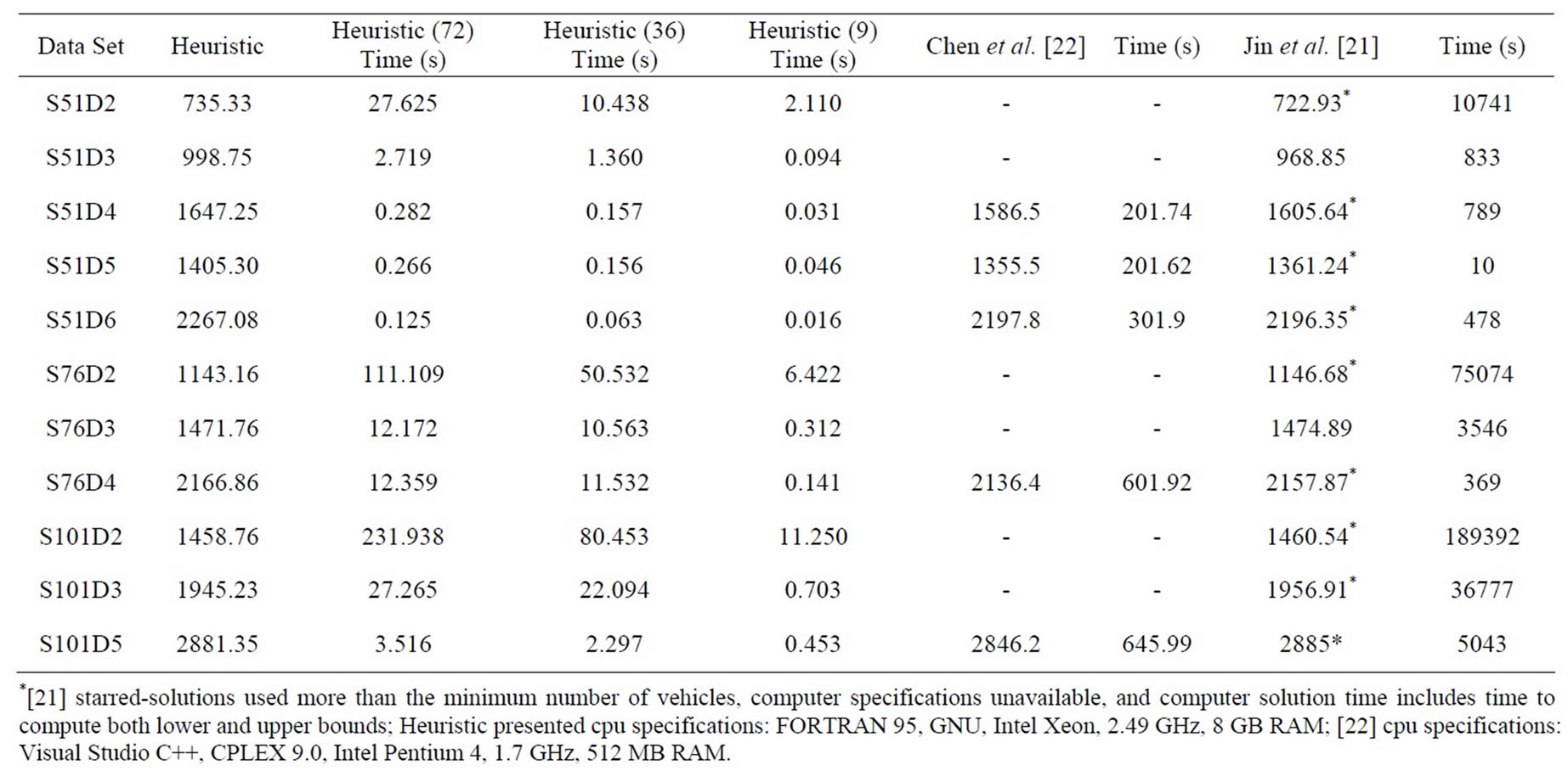
Table 4. Comparing the construction heuristic versus [21,22] for 11 data sets.
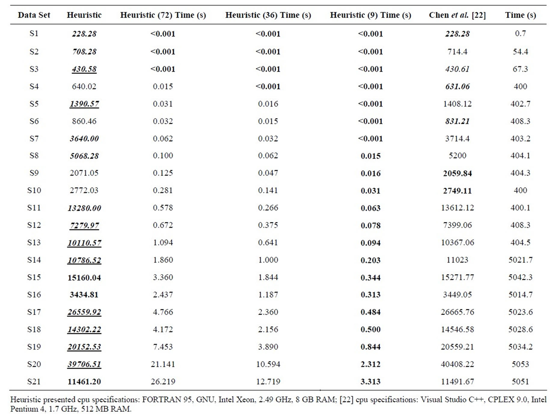
Table 5. Comparing the results of the construction heuristic versus the two-phase method of [22] for 21 data sets.
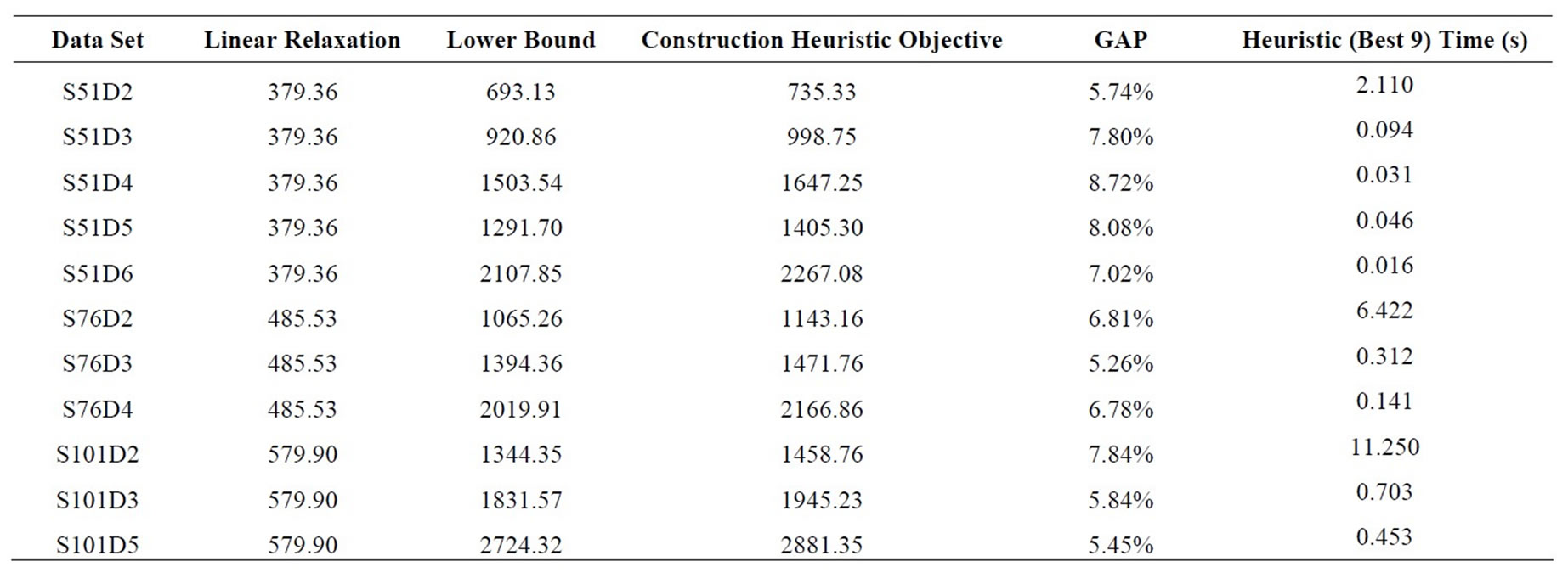
Table 6. Duality GAP for construction heuristic solution for 11 data sets. Lower bounds from [21].
generation [21], the two-step method developed by Chen et al. [22], and a neighborhood search [26]. The construction heuristic does not assume symmetric distances, and a future research direction would be to test this heuristic with asymmetric data sets.
REFERENCES
- G. B. Dantzig and J. H. Ramser, “The Truck Dispatching Problem,” Management Science, Vol. 6, No. 1, 1959, pp. 80-91. doi:10.1287/mnsc.6.1.80
- P. Toth and D. Vigo, “The Vehicle Routing Problem,” Society for Industrial and Applied Mathematics, Philadelphia, 2002.
- P. Toth and D. Vigo, “Models, Relaxations and Exact Approaches for the Capacitated Vehicle Routing Problem,” Discrete Applied Mathematics, Vol. 123, No. 1-3, 2002, pp. 487-512. doi:10.1016/S0166-218X(01)00351-1
- J. F. Cordeau, M. Gendreau, G. Laporte, J.-Y. Potvin and F. Semet, “A Guide to Vehicle Routing Heuristics,” Journal of the Operational Research Society, Vol. 53, 2002, pp. 512-522. doi:10.1057/palgrave.jors.2601319
- J. F. Cordeau, M. Gendreau, A. Hertz, G. Laporte and J. S. Sormany, “New Heuristics for the Vehicle Routing Problem,” In: A. Langevin and D. Riopel, Eds., Logistics Systems: Design and Optimization, Springer, 2005, pp. 270- 297. doi:10.1007/0-387-24977-X_9
- M. Dror and P. Trudeau, “Savings by Split Delivery Routing,” Transportation Science, Vol. 23, No. 2, 1989, pp. 141-145. doi:10.1287/trsc.23.2.141
- M. Dror and P. Trudeau, “Split Delivery Routing,” Naval Research Logistics, Vol. 37, 1990, pp. 383-402.
- M. Dror, G. Laporte and P. Trudeau, “Vehicle Routing with Split Deliveries,” Discrete Applied Mathematics, Vol. 50, No. 3, 1994, pp. 239-254. doi:10.1016/0166-218X(92)00172-I
- C. Archetti and M. G. Speranza, “An Overview on the Split Delivery Vehicle Routing Problem,” Operations Research Proceedings, Part IV, 2006, pp. 123-127.
- C. Archetti and M. G. Speranza, “The Split Delivery Vehicle Routing Problem: A Survey. The Vehicle Routing Problem: Latest Advances and New Challenges,” Operations Research/Computer Science Interfaces Series, Vol. 43, Part I, 2008, pp. 103-122. doi:10.1016/0166-218X(92)00172-I
- D. J. Gulczynski, B. Golden and E. Wasil, “Recent Developments in Modeling and Solving the Split Delivery Vehicle Routing Problem,” Tutorials in Operations Research, INFORMS, 2008, pp. 170-180.
- B. L. Golden and A. A. Assad, “Vehicle Routing: Methods and Studies,” North-Holland, Amsterdam, 1988.
- P. W. Frizzell and J. W. Giffin, “The Split Delivery Vehicle Scheduling Problem with Time Windows and Grid Network Distances,” Computers and Operations Research, Vol. 22, No. 6, 1995, pp. 655-667. doi:10.1016/0305-0548(94)00040-F
- P. W. Frizzell and J. W. Giffin, “The Bounded Split Delivery Vehicle Routing Problem with Grid Network Distances,” Asia Pacific Journal of Operational Research, Vol. 9, 1992, pp. 101-116.
- C. Archetti, M. Savelsbergh and A. Hertz, “A Tabu Search Algorithm for the Split Delivery Vehicle Routing Problem,” Transportation Science, Vol. 40, No. 1, 2006, pp. 64-73. doi:10.1287/trsc.1040.0103
- C. Archetti, M. Savelsbergh and M. G. Speranza, “WorstCase Analysis for Split Delivery Vehicle Routing Problems,” Transportation Science, Vol. 40, No. 2, 2006, pp. 226-234. doi:10.1287/trsc.1050.0117
- C. Archetti, M. Savelsbergh and M. G. Speranza, “To Split or Not to Split: That Is the Question,” Transportation Research Part E, Vol. 44, No. 1, 2008, pp. 114-123. doi:10.1016/j.tre.2006.04.003
- C. Lee, M. A. Epelman, C. C. White and Y. A. Bozer, “A Shortest Path Approach to the Multiple-Vehicle Routing Problem with Split Pick-Ups,” Transportation Research Part B, Vol. 40, No. 4, 2006, pp. 265-284. doi:10.1016/j.trb.2004.11.004
- J. M. Belenguer, M. C. Martinez and E. A. Mota, “Lower Bound for the Split Delivery VRP,” Operations Research, Vol. 48, No. 5, 2000, pp. 801-810. doi:10.1287/opre.48.5.801.12407
- M. Jin, K. Liu and R. O. Bowden, “A Two-Stage Algorithm with Valid Inequalities for the Split Delivery Vehicle Routing Problem,” International Journal of Production Economics, Vol. 105, No. 1, 2007, pp. 228-242. doi:10.1016/j.ijpe.2006.04.014
- M. Jin, K. Liu and B. Eksioglu, “A Column Generation Algorithm for the Vehicle Routing Problem with Split Delivery,” Proceedings of the 2007 Industrial Engineering Research Conference, Nashville, 19-23 May 2007.
- S. Chen, B. Golden and E. Wasil, “The Split Delivery Vehicle Routing Problem: Applications, Test Problems, and Computational Results,” Networks, Vol. 94, No. 4, 2007, pp. 318-329. doi:10.1002/net.20181
- S. Chen, “A Study of Four Network Problems in Transportation, Telecommunications, and Supply Chain Management,” Dissertation Thesis, University of Maryland, 2007.
- G. Clarke and J. Wright, “Scheduling of Vehicles from a Central Depot to a Number of Delivery Points,” Operations Research, Vol. 12, No. 4, 1964, pp. 568-581. doi:10.1287/opre.12.4.568
- W. Burrows, “The Vehicle Routing Problem with Loadsplitting: A Heuristic Approach,” 24th Annual Conference of the Operational Research Society of New Zealand, 1988, pp. 33-38.
- R. E. Aleman, “A Guided Neighborhood Search Applied to the Split Delivery Vehicle Routing Problem,” Dissertation Thesis, Wright State University, 2009.
- K. Liu, “A Study on the Split Delivery Vehicle Routing Problem,” Dissertation Thesis, Mississippi State University, 2005.
- M. A. Nowak, “The Pickup and Delivery Problem with Split Loads,” Dissertation Thesis, Georgia Institute of Technology, 2005.
- J. H. Wilck IV, “Solving the Split Delivery Vehicle Routing Problem,” Dissertation Thesis, Pennsylvania State University, 2009.
- P. Mullaseril, M. Dror and J. Leung, “Split-Delivery Routing Heuristics in Livestock Feed Distribution,” Journal of the Operational Research Society, Vol. 48, 1997, pp. 107-116.
- G. Sierksma and G. A. Tijssen, “Routing Helicopters for Crew Exchanges on Off-Shore Locations,” Annals of Operations Research, Vol. 76, 1998, pp. 261-286. doi:10.1023/A:1018900705946
- S. Song, K. Lee and G. Kim, “A Practical Approach to Solving a Newspaper Logistics Problem Using a Digital Map,” Computers and Industrial Engineering, Vol. 43, No. 1-2, 2002, pp. 315-330. doi:10.1016/S0360-8352(02)00077-3
- M. M. Syslo, N. Deo and J. S. Kowalik, “Discrete Optimization Algorithms with PASCAL Programs,” PrenticeHall, Englewood Cliffs, 1983.