Modern Economy, 2010, 1, 1-16
doi:10.4236/me.2010.11001 Published Online May 2010 (http://www.SciRP.org/journal/me)
Dynamic Interactive Cycles during the 2008 Financial Crisis
Ioannis M. Neokosmidis, Vassilis Polimenis
Department of Economics, Aristotle University of Thessaloniki, Thessaloniki, Greece
Received February 16, 2010; revised March 20, 2010; accepted March 30, 2010
Abstract
This paper focuses on the analysis of the 2008 financial crisis and how it affects the global financial markets.
We analyze three major markets (US, UK, and ASIA) that are represented by the levels of three broad stock
indices S&P 500, FTSE 100 and Hang Seng respectively. Our methodology is based on cointegration analy-
sis and Granger causality test in order to examine the interaction between the markets (information flows).
Additionally, we study the volatility transmission based on multivariate GARCH analysis. We find significant
changes in information flows before and during the financial crisis.
Keywords: Unit Root Test, Cointegration, Granger Causality, Multivariate Volatility Processes, Financial
Crisis
1. Introduction
Due to its surprising breadth and intensity, the analysis of
the 2008 global financial crisis presents a major challenge
for economists and financial experts. Policymakers now
consider the definition of key policy responses and institu-
tional rules in order to build mechanisms that will contain
cross-market contagion and prevent a reoccurrence of the
problem in the future. Most of the recent crises1 started
from emerging markets, which are presumably more sen-
sitive to liquidity shocks because of their underdeveloped
and illiquid financial markets and their large public defi-
cits. Besides the 1987 crash in Wall Street that was tech-
nical and short-lived in nature, the 2008 crisis is the first to
be labelled a US crisis on the basis that it seems to have
started by the massive US real estate delinquencies.
An important question related to an international finan-
cial crisis is the existence of contagion (i.e., the interna-
tional propagation of country- or region-specific shocks to
other parts of the world). According to the more open
definition adopted by Forbes and Rigobon [1], contagion
is measured as any change in the transmission mecha-
nisms that occurs during a volatile period. For example,
contagion may establish itself by a significant increase in
cross-market correlations.
Yet to date, there is still a lot of disagreement as to what
are the channels through which financial upheaval is
transmitted across countries, and on the set of measurable
factors that may be used for the precise identification of a
contagion event. Understanding these factors is important
because early recognition of the possibility of contagion
may help reduce a country’s vulnerability to externally-
originated shocks.
In the wake of the current financial international crash,
growing integration of financial markets has been of heig-
htened interest because such integration is assumed to
generate large, correlated price movements across most
stock markets. Yet due to the complexity and global nature
of the current financial crisis, it is difficult to move beyond
the headlines of the financial press and provide an in depth
analysis of the mechanism that links global financial mar-
kets during the crisis and generates the phenomenon of
contagion.
The analysis may take place on both the economics of
the crisis, as well as on a purely statistical manner. On the
economic front, in the US for example, the fight has pro-
duced what is termed “a highly accommodative monetary
policy.” What is truly meant by this deceptively soft phr-
ase is that since the onset of the financial crisis nearly two
years ago, the Federal Reserve has reduced the cost of
funds for big US banks nearly to zero. This has happened
by adjusting the interest-rate target for overnight lending
between banks (the so called Fed-funds rate).
1The most well known financial and currency crises that have occurred
over the last 25 years with global consequences were, the 1992 Euro-
p
ean monetary unit problems, the peso effect of 1994, and the 1997
Asian “flu” crisis (which also triggered the 1998 Russian “cold”). The
1999 Brazilian devaluation, the 2000 Internet bubble burst, and the
Jul
y
2001 default of Ar
g
entina.
Having brought the Fed-funds rate to almost zero, the
US (and later the UK) switched to the more aggressive
policy of Quantitative Easing, which is also described as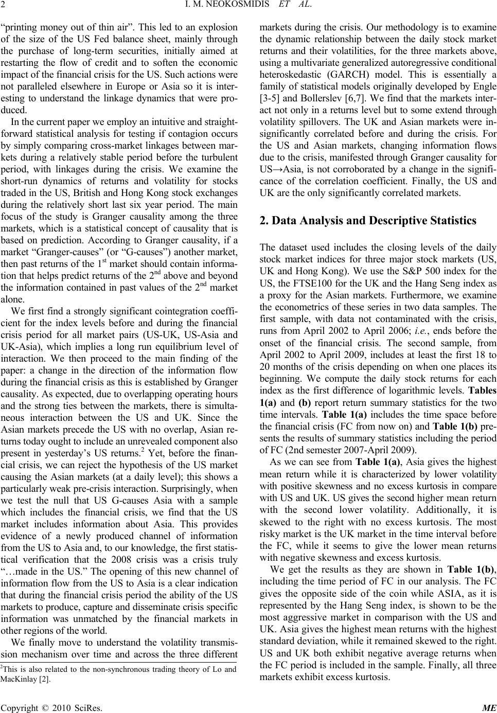

I. M. NEOKOSMIDIS ET AL. 2
“printing money out of thin air”. This led to an explosion
of the size of the US Fed balance sheet, mainly through
the purchase of long-term securities, initially aimed at
restarting the flow of credit and to soften the economic
impact of the financial crisis for the US. Such actions were
not paralleled elsewhere in Europe or Asia so it is inter-
esting to understand the linkage dynamics that were pro-
duced.
In the current paper we employ an intuitive and straight-
forward statistical analysis for testing if contagion occurs
by simply comparing cross-market linkages between mar-
kets during a relatively stable period before the turbulent
period, with linkages during the crisis. We examine the
short-run dynamics of returns and volatility for stocks
traded in the US, British and Hong Kong stock exchanges
during the relatively short last six year period. The main
focus of the study is Granger causality among the three
markets, which is a statistical concept of causality that is
based on prediction. According to Granger causality, if a
market “Granger-causes” (or “G-causes”) another market,
then past returns of the 1st market should contain informa-
tion that helps predict returns of the 2nd above and beyond
the information contained in past values of the 2nd market
alone.
We first find a strongly significant cointegration coeffi-
cient for the index levels before and during the financial
crisis period for all market pairs (US-UK, US-Asia and
UK-Asia), which implies a long run equilibrium level of
interaction. We then proceed to the main finding of the
paper: a change in the direction of the information flow
during the financial crisis as this is established by Granger
causality. As expected, due to overlapping operating hours
and the strong ties between the markets, there is simulta-
neous interaction between the US and UK. Since the
Asian markets precede the US with no overlap, Asian re-
turns today ought to include an unrevealed component also
present in yesterday’s US returns.2 Yet, before the finan-
cial crisis, we can reject the hypothesis of the US market
causing the Asian markets (at a daily level); this shows a
particularly weak pre-crisis interaction. Surprisingly, when
we test the null that US G-causes Asia with a sample
which includes the financial crisis, we find that the US
market includes information about Asia. This provides
evidence of a newly produced channel of information
from the US to Asia and, to our knowledge, the first statis-
tical verification that the 2008 crisis was a crisis truly
“…made in the US.” The opening of this new channel of
information flow from the US to Asia is a clear indication
that during the financial crisis period the ability of the US
markets to produce, capture and disseminate crisis specific
information was unmatched by the financial markets in
other regions of the world.
We finally move to understand the volatility transmis-
sion mechanism over time and across the three different
markets during the crisis. Our methodology is to examine
the dynamic relationship between the daily stock market
returns and their volatilities, for the three markets above,
using a multivariate generalized autoregressive conditional
heteroskedastic (GARCH) model. This is essentially a
family of statistical models originally developed by Engle
[3-5] and Bollerslev [6,7]. We find that the markets inter-
act not only in a returns level but to some extend through
volatility spillovers. The UK and Asian markets were in-
significantly correlated before and during the crisis. For
the US and Asian markets, changing information flows
due to the crisis, manifested through Granger causality for
US→Asia, is not corroborated by a change in the signifi-
cance of the correlation coefficient. Finally, the US and
UK are the only significantly correlated markets.
2. Data Analysis and Descriptive Statistics
The dataset used includes the closing levels of the daily
stock market indices for three major stock markets (US,
UK and Hong Kong). We use the S&P 500 index for the
US, the FTSE100 for the UK and the Hang Seng index as
a proxy for the Asian markets. Furthermore, we examine
the econometrics of these series in two data samples. The
first sample, with data not contaminated with the crisis,
runs from April 2002 to April 2006; i.e., ends before the
onset of the financial crisis. The second sample, from
April 2002 to April 2009, includes at least the first 18 to
20 months of the crisis depending on when one places its
beginning. We compute the daily stock returns for each
index as the first difference of logarithmic levels. Tables
1(a) and (b) report return summary statistics for the two
time intervals. Table 1(a) includes the time space before
the financial crisis (FC from now on) and Table 1(b) pre-
sents the results of summary statistics including the period
of FC (2nd semester 2007-April 2009).
As we can see from Table 1(a), Asia gives the highest
mean return while it is characterized by lower volatility
with positive skewness and no excess kurtosis in compare
with US and UK. US gives the second higher mean return
with the second lower volatility. Additionally, it is
skewed to the right with no excess kurtosis. The most
risky market is the UK market in the time interval before
the FC, while it seems to give the lower mean returns
with negative skewness and excess kurtosis.
We get the results as they are shown in Table 1(b),
including the time period of FC in our analysis. The FC
gives the opposite side of the coin while ASIA, as it is
represented by the Hang Seng index, is shown to be the
most aggressive market in comparison with the US and
UK. Asia gives the highest mean returns with the highest
standard deviation, while it remained skewed to the right.
US and UK both exhibit negative average returns when
the FC period is included in the sample. Finally, all three
markets exhibit excess kurtosis.
2This is also related to the non-synchronous trading theory of Lo and
MacKinlay [2].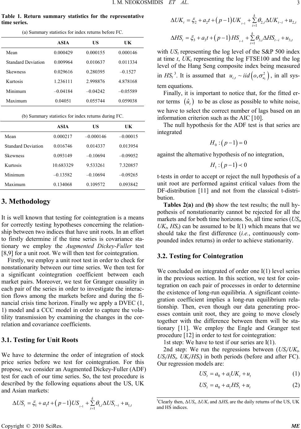

I. M. NEOKOSMIDIS ET AL.3
Table 1. Return summary statistics for the representative
time series.
(a) Summary statistics for index returns before FC.
ASIA US UK
Mean 0.000429 0.000155 0.000146
Standard Deviation 0.009964 0.010637 0.011334
Skewness 0.029616 0.280395 –0.1527
Kurtosis 1.236111 2.998876 4.878168
Minimum –0.04184 –0.04242 –0.05589
Maximum 0.04051 0.055744 0.059038
(b) Summary statistics for index returns during FC.
ASIA US UK
Mean 0.000217 –0.000146 –0.00015
Standard Deviation 0.016746 0.014337 0.013954
Skewness 0.093149 –0.10694 –0.09052
Kurtosis 10.683329 9.533261 7.320857
Minimum –0.13582 –0.10694 –0.09265
Maximum 0.134068 0.109572 0.093842
3. Methodology
It is well known that testing for cointegration is a means
for correctly testing hypotheses concerning the relation-
ship between two indices that have unit roots. In an effort
to firstly determine if the time series is covariance sta-
tionary we employ the Augmented Dickey-Fuller test
[8,9] for a unit root. We will then test for cointegration.
Firstly, we employ a unit root test in order to check for
nonstationarity between our time series. We then test for
a significant cointegration coefficient between each
market pairs. Moreover, we test for Granger causality in
each pair of the series in order to investigate the interac-
tion flows among the markets before and during the fi-
nancial crisis time horizon. Finally we apply a DVEC (1,
1) model and a CCC model in order to capture the vola-
tility transmission by examining the changes in the cor-
relation and covariance coefficients.
3.1. Testing for Unit Roots
We have to determine the order of integration of stock
price series before we test for cointegration. For this
propose, we consider an Augmented Dickey-Fuller (ADF)
test for each of our time series. So, the test procedure is
described by the following equations about the US, UK
and Asian markets:

1
111, 1,
1
1t
k
t
i
USa tpUSUSu 


 
i
tit
tit
tit

1
222, 2,
1
1t
k
ti
i
UKa tpUKUKu 


 


1
3 33,3,
1
1t
k
ti
i
H
Sa tpHSHSu 


  

with USt representing the log level of the S&P 500 index
at time t, UKt representing the log FTSE100 and the log
level of the Hang Seng composite index being measured
in HSt
3. It is assumed that

2
,~,
i
it u
uiido


, in all sys-
tem equations.
Finally, it is important to notice that, for the fitted er-
ror terms


ˆt u to be as close as possible to white noise,
we have to select the correct number of lags based on an
information criterion such as the AIC [10].
The null hypothesis for the ADF test is that series are
integrated


0:1Hp0
against the alternative hypothesis of no integration,


1:1Hp0
tt
t-tests in order to accept or reject the null hypothesis of a
unit root are performed against critical values from the
DF-distribution [11] and not from the classical t-distri-
bution.
Tables 2(a) and (b) show the test results; the null hy-
pothesis of nonstationarity cannot be rejected for all the
markets and for both time horizons. So, all time series (USt,
UKt, HSt) can be assumed to be I(1) which means that we
should take the first difference (i.e., continuously com-
pounded index returns) in order to achieve stationarity.
3.2. Testing for Cointegration
We concluded on integrated of order one I(1) level series
in the previous section. In this section, we test for coin-
tegration on each pair of processes in order to determine
the existence of long-run equilibria. A significant cointe-
gration coefficient implies a long-run equilibrium rela-
tionship. Then, even though our data generating proc-
esses contain unit root, they are going to move closely
together with the difference between them will be sta-
tionary [11]. We employ the Engle and Granger test
procedure [12] in order to test for cointegration:
1st step: We have to test if our series are I(1).
2nd step: We run the regressions between (USt/UKt,
USt/HSt, UKt/HSt) in both periods (before and after FC).
Our regression models are:
01t
USaa UKu

 (1)
01t
USaa HSu
tt

 (2)
3Clearly then, ΔUSt, ΔUKt and ΔHSt are the daily returns of the US, UK
and HS indices.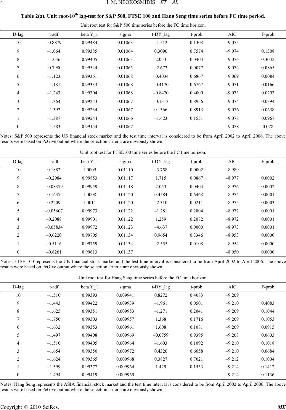

I. M. NEOKOSMIDIS ET AL. 4
Table 2(a). Unit root-10th lag-test for S&P 500, FTSE 100 and Hang Seng time series before FC time period.
Unit root test for S&P 500 time series before the FC time horizon.
D-lag t-adf beta Y_1 sigma t-DY_lag t-prob AIC F-prob
10 –0.8879 0.99484 0.01063 –1.512 0.1308 –9.075
9 –1.064 0.99385 0.01064 0.3090 0.7574 –9.074 0.1308
8 –1.036 0.99405 0.01063 2.053 0.0403 –9.076 0.3042
7 –0.7980 0.99544 0.01065 –2.672 0.0077 –9.074 0.0865
6 –1.123 0.99361 0.01068 –0.4034 0.6867 –9.069 0.0084
5 –1.181 0.99333 0.01068 –0.4170 0.6767 –9.071 0.0166
4 –1.243 0.99304 0.01068 –0.8420 0.4000 –9.073 0.0293
3 –1.364 0.99243 0.01067 –0.1313 0.8956 –9.074 0.0394
2 –1.392 0.99234 0.01067 0.1366 0.8913 –9.076 0.0638
1 –1.387 0.99244 0.01066 –1.423 0.1551 –9.078 0.0967
0 –1.583 0.99144 0.01067 –9.078 0.078
Notes: S&P 500 represents the US financial stock market and the test time interval is considered to be from April 2002 to April 2006. The above
results were based on PcGive output where the selection criteria are obviously shown.
Unit root test for FTSE100 time series before the FC time horizon.
D-lag t-adf beta Y_1 sigma t-DY_lag t-prob AIC F-prob
10 0.1882 1.0009 0.01110 –3.758 0.0002 –8.989
9 –0.2984 0.99853 0.01117 1.715 0.0867 –8.977 0.0002
8 –0.08379 0.99959 0.01118 2.053 0.0404 –8.976 0.0002
7 0.1637 1.0008 0.01120 0.4584 0.6468 –8.974 0.0001
6 0.2209 1.0011 0.01120 –2.310 0.0211 –8.975 0.0003
5 –0.05607 0.99973 0.01122 –1.281 0.2004 –8.972 0.0001
4 –0.2088 0.99901 0.01122 1.259 0.2082 –8.972 0.0001
3 –0.05834 0.99972 0.01123 –4.637 0.0000 –8.973 0.0001
2 –0.6220 0.99705 0.01134 0.9654 0.3346 –8.953 0.0000
1 –0.5116 0.99759 0.01134 –2.555 0.0108 –8.954 0.0000
0 –0.8261 0.99613 0.01137 –8.950 0.0000
Notes: FTSE 100 represents the UK financial stock market and the test time interval is considered to be from April 2002 to April 2006. The above
results were based on PcGive output where the selection criteria are obviously shown.
Unit root test for Hang Seng time series before the FC time horizon.
D-lag t-adf beta Y_1 sigma t-DY_lag t-prob AIC F-prob
10 –1.510 0.99393 0.009941 0.8272 0.4083 –9.209
9 –1.443 0.99422 0.009939 –1.961 0.0501 –9.210 0.4083
8 –1.625 0.99351 0.009953 –1.271 0.2041 –9.209 0.1044
7 –1.750 0.99303 0.009957 1.368 0.1716 –9.209 0.1053
6 –1.632 0.99353 0.009961 1.608 0.1081 –9.209 0.0915
5 –1.497 0.99408 0.009969 –0.0759 0.9395 –9.208 0.0603
4 –1.510 0.99405 0.009964 –1.603 0.1092 –9.210 0.1018
3 –1.654 0.99350 0.009972 0.4320 0.6658 –9.210 0.0684
2 –1.624 0.99365 0.009968 0.3827 0.7021 –9.212 0.1004
1 –1.599 0.99377 0.009964 1.429 0.1533 –9.214 0.1412
0 –1.494 0.99419 0.009969 –9.214 0.1136
Notes: Hang Seng represents the ASIA financial stock market and the test time interval is considered to be from April 2002 to April 2006. The above
results were based on PcGive output where the selection criteria are obviously shown.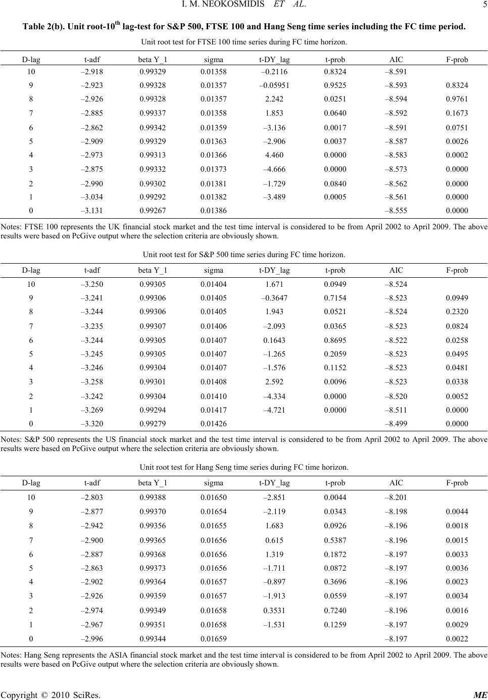

I. M. NEOKOSMIDIS ET AL.5
Table 2(b). Unit root-10th lag-test for S&P 500, FTSE 100 and Hang Seng time series including the FC time period.
Unit root test for FTSE 100 time series during FC time horizon.
D-lag t-adf beta Y_1 sigma t-DY_lag t-prob AIC F-prob
10 –2.918 0.99329 0.01358 –0.2116 0.8324 –8.591
9 –2.923 0.99328 0.01357 –0.05951 0.9525 –8.593 0.8324
8 –2.926 0.99328 0.01357 2.242 0.0251 –8.594 0.9761
7 –2.885 0.99337 0.01358 1.853 0.0640 –8.592 0.1673
6 –2.862 0.99342 0.01359 –3.136 0.0017 –8.591 0.0751
5 –2.909 0.99329 0.01363 –2.906 0.0037 –8.587 0.0026
4 –2.973 0.99313 0.01366 4.460 0.0000 –8.583 0.0002
3 –2.875 0.99332 0.01373 –4.666 0.0000 –8.573 0.0000
2 –2.990 0.99302 0.01381 –1.729 0.0840 –8.562 0.0000
1 –3.034 0.99292 0.01382 –3.489 0.0005 –8.561 0.0000
0 –3.131 0.99267 0.01386 –8.555 0.0000
Notes: FTSE 100 represents the UK financial stock market and the test time interval is considered to be from April 2002 to April 2009. The above
results were based on PcGive output where the selection criteria are obviously shown.
Unit root test for S&P 500 time series during FC time horizon.
D-lag t-adf beta Y_1 sigma t-DY_lag t-prob AIC F-prob
10 –3.250 0.99305 0.01404 1.671 0.0949 –8.524
9 –3.241 0.99306 0.01405 –0.3647 0.7154 –8.523 0.0949
8 –3.244 0.99306 0.01405 1.943 0.0521 –8.524 0.2320
7 –3.235 0.99307 0.01406 –2.093 0.0365 –8.523 0.0824
6 –3.244 0.99305 0.01407 0.1643 0.8695 –8.522 0.0258
5 –3.245 0.99305 0.01407 –1.265 0.2059 –8.523 0.0495
4 –3.246 0.99304 0.01407 –1.576 0.1152 –8.523 0.0481
3 –3.258 0.99301 0.01408 2.592 0.0096 –8.523 0.0338
2 –3.242 0.99304 0.01410 –4.334 0.0000 –8.520 0.0052
1 –3.269 0.99294 0.01417 –4.721 0.0000 –8.511 0.0000
0 –3.320 0.99279 0.01426 –8.499 0.0000
Notes: S&P 500 represents the US financial stock market and the test time interval is considered to be from April 2002 to April 2009. The above
results were based on PcGive output where the selection criteria are obviously shown.
Unit root test for Hang Seng time series during FC time horizon.
D-lag t-adf beta Y_1 sigma t-DY_lag t-prob AIC F-prob
10 –2.803 0.99388 0.01650 –2.851 0.0044 –8.201
9 –2.877 0.99370 0.01654 –2.119 0.0343 –8.198 0.0044
8 –2.942 0.99356 0.01655 1.683 0.0926 –8.196 0.0018
7 –2.900 0.99365 0.01656 0.615 0.5387 –8.196 0.0015
6 –2.887 0.99368 0.01656 1.319 0.1872 –8.197 0.0033
5 –2.863 0.99373 0.01656 –1.711 0.0872 –8.197 0.0036
4 –2.902 0.99364 0.01657 –0.897 0.3696 –8.196 0.0023
3 –2.926 0.99359 0.01657 –1.913 0.0559 –8.197 0.0034
2 –2.974 0.99349 0.01658 0.3531 0.7240 –8.196 0.0016
1 –2.967 0.99351 0.01658 –1.531 0.1259 –8.197 0.0029
0 –2.996 0.99344 0.01659 –8.197 0.0022
Notes: Hang Seng represents the ASIA financial stock market and the test time interval is considered to be from April 2002 to April 2009. The above
esults were based on PcGive output where the selection criteria are obviously shown. r

I. M. NEOKOSMIDIS ET AL. 6
tt
t
01t
UKaa HSu  (3)
3rd step: We obtain the fitted errors

from the
above regressions and we test if they include any sto-
chastic trends or not. Then, if we find unit roots in the
residuals we conclude that there is no cointegration be-
tween the series. So, we apply an ADF test in the fitted
errors,

ˆt
u
11
ˆˆ ˆ
k
tt iti
i
uau bu



 
 (4)
where the null is:
0:0Ha

against the alternative,
1:0Ha
The results are shown in Tables 3 and 4, where we re-
ject the null (no cointegration) at all lags for all market
pairs. The financial crisis does not affect the existence of
long-run relationship among the three markets.
3.3. Information Flow
Even if the financial crisis did not affect the long-run
relationship of the markets, it may still have affected the
flow of information (the direction of interaction) between
them. As we discussed already, we find cointegration
between (US/UK), (US/HS) and (UK/HS) markets. Yet,
we don’t know the direction of information flow (direc-
tion of interaction) between the markets.
As is well known Granger causality from X to Y does
not indicate causality in the proper common use of the
term (i.e., it does not imply that the Y series is the effect
or the result of X series). Instead, Granger causality truly
measures precedence and information flow, so that in our
context here of the recent financial crisis Granger causal-
ity from a country X to country Y implies that informa-
tion during the crisis flows from X to Y. Alternatively,
we may think of developments in X preceding develop-
ments in Y.
Our aim in this section is to describe the dynamic in-
teraction between the markets and to see the independent
movements before we proceed to volatility modelling. It
is a crucial aspect of a proper analysis of the crisis to
analyze the cycle of information before we move to the
next level of volatility analysis.
We separate our markets in three bi-variate VAR proc-
esses [13] like following:
11,1 11,211
22,1 12,212
ttt
ttt
USc UScUKv
UKc UScUKv




 



 


t
t
t
t



t
t
(5)
11,111,2 11
22,112,2 12
ttt
ttt
UKc UKcHS
HSc UKcHS





 










(7)
Alternatively, in the absence of Granger causality, our
series are generated by an AR(1) process as follows:
11 11tt
USap USu
t

  (8)
22 1tt2t
H
SapHS u


  (9)
33 13tt
UKap UKu
t

  (10)
We say that (Ri,t ) return series does not Granger cause
(G-cause) the (Rj,t ) return series if and only if the best
linear prediction of Rj,t given the information set { Ri,t-1,
Rj,t-1) does not depend on Ri,t-1.
Following the above modelling, we can test the null
hypothesis against the alternative:
UK does not G-cause US:
01,2
11,2
:0
:0
Hc
Hc


or alternatively, we may say that under the null hypothe-
sis the residual variances in (5) and (8) above are the
same since ΔUKt-1 does not have any significance in ex-
plaining ΔUSt, i.e.
22
01 1
22
11 1
:()()
:()()
tt
tt
H
Ev Eu
H
Ev Eu


US does not G-cause UK:
02,1
12,1
:0
:0
Hc
Hc


or
22
02 3
22
12 3
:( )( )
:( )( )
tt
tt
H
Ev Eu
H
Ev Eu


HS does not G-cause US:
012
112
:0
:0
Hc
Hc


，
，
or
22
01 1
22
11 1
:( )( )
:( )( )
tt
tt
H
EEu
H
EEu




US does not G-cause HS:
02,1
12,1
:0
:0
Hc
Hc


or
22
02 2
22
12 2
:( )( )
:( )( )
tt
tt
H
EEu
H
EEu




HS does not G-cause UK:
01,2
11,2
:0
:0
Hc
Hc


or
22
01 3
22
11 3
:( )()
:( )()
tt
tt
H
EEu
H
EEu




UK does not G-cause HS:
02,1
12,1
:0
:0
Hc
Hc


or
22
02 2
22
12 2
:( )()
:( )()
tt
tt
H
EEu
H
EEu




11,111,21 1
22,112,212
ttt
ttt
USc UScHS
HSc UScHS




  



  


(6)
3.3.1. Estimation and Testing
We have already described an assumed regression
structure for our series. We perform maximum likelihood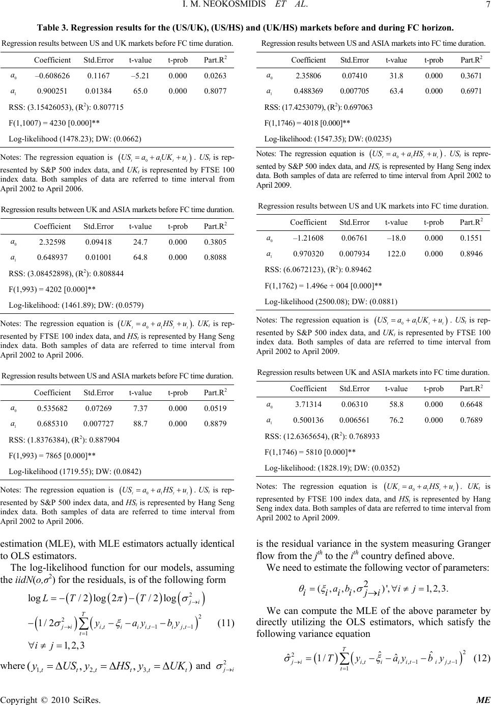

I. M. NEOKOSMIDIS ET AL.7
and (on. Table 3. Regression results for the (US/UK), (US/HS)
Regression
UK/HS) markets before and during FC horiz
results between US and UK markets before FC time duration.
2
Coefficient Std.Error t-value t-prob Part.R
0
a –0.608626 0.1167 –5.21 0.000 0.0263
1
a 0.900251 0.01384 65.0 0.000 0.8077
RSS: (3., (R2
: (0.0662)
15426053) ): 0.807715
F( 1007) = 4230 [0.000]** 1,
Log-likelihood (1478.23); DW
Ν

is rep-
resented by S&P 500 index data, 100
d ASIA markets before FC time duration.
2
otes: Τhe regression equation is

t
US a
01t
a UKu .
and UKt is represented by
are referred to time in
t
USt
FTSE
index data. Both samples of data terval from
April 2002 to April 2006.
Regression results between UK an
Coefficient Std.Error t-value t-prob Part.R
0
a 2.32598 0.09418 24.7 0.000 0.3805
1
a 0.
RSS: (3., (R2
: (0.0579)
648937 0.01001 64.8 0.000 0.8088
08452898) ): 0.808844
F( 993) = 4202 [0.000]** 1,
Log-likelihood: (1461.89); DW
Ν 
t
UKt is rep-
resented by FTSE 100 index data, and HSt is represented by Hang Seng
are referred to time
nd ASIA markets before FC time duration.
2
otes: Τhe regression equation is 
01t
UK at a HSu .
index data. Both samples of data interval from
April 2002 to April 2006.
Regression results between US a
Coefficient Std.Error t-value t-prob Part.R
0
a 0.535682 0.07269 7.37 0.000 0.0519
1
a 0.685310 0.007727 88.7 0.000 0.8879
RSS: (1.R2
: (0.0842)
8376384), (): 0.887904
F( 993) = 7865 [0.000]** 1,
Log-likelihood (1719.55); DW
Ν

is rep-
resented by S&P 500 index data,
ation.
Coe2
otes: Τhe regression equation is

t
US a
01t
a HSu .
and HSt is represented by Hang Seng
are referred to time in
t
USt
index data. Both samples of data terval from
April 2002 to April 2006.
Regression results between US and ASIA markets into FC time dur
fficientStd.Error t-value t-prob Part.R
0
a 2.35806 0.07410 31.8 0.000 0.3671
1
a 0 0
RSS: (17. (R2): 0
: (0.0235)
.488369.00770563.4 0.000 0.6971
4253079), .697063
F( 746) = 4018 [0.000]** 1,1
Log-likelihood: (1547.35); DW
Νotes: Τhe regression equation is


01t
USaa HSu .
t
nted by S&P 500 index data, and HSt is re
t
USt is repre-
se presented by Hang Seng index
ed to time interval from
results between US and UK markets into FC time duration.
2
data. Both samples of data are referr April 2002 to
April 2009.
Regression
CoefficientStd.Error t-value t-prob Part.R
0
a –1.216080.06761 –18.0 0.000 0.1551
1
a 0.970320 0.
RSS: (6., (R2
**
007934122.0 0.000 0.8946
0672123) ): 0.89462
F( 1762) = 1.496e + 004 [0.000]1,
Log-likelihood (2500.08); DW: (0.0881)
Νt US
resented by S&P 500 index data,
2
otes: Τhe regression equation is

t
US a

t is rep-
FTSE 100
01t
a UKu .
and UKt is represented by
are referred to time iindex data. Both samples of data nterval from
April 2002 to April 2009.
Regression results between UK and ASIA markets into FC time duration.
CoefficientStd.Error t-value t-prob Part.R
0
a 3.71314 0.06310 58.8 0.000 0.6648
1
a 0. 0.
RSS: (12.), (R2
: (0.0352)
50013600656176.2 0.000 0.7689
6365654): 0.768933
F( 1746) = 5810 [0.000]** 1,
Log-likelihood: (1828.19); DW
Ν

t
UKt is
represented by FTSE 100 index data, and HSt is represented by Hang
ta are referred to time
th MLE estimators actually identical
OLS estimators.
residuals, is of the following form
1
otes: Τhe regression equation is

t
UK 01t aa HSu .
Seng index data. Both samples of da interval from
April 2002 to April 2009.
estimation (MLE), wi
to
The log-likelihood function for our models, assuming
the iidN(o,σ2) for the


2
log/2log2 /2log

 
2
2
,, 1,
1
1/2
1, 2,3
j
i
LT T 

 
T
jiitii itijt
t
ya yby
ij



 
 

(11)
where and
),,(,3,2,1 tttttt UKyHSyUSy 
2
j
i


is the residual variance in the system measuring Granger
flow from the jth to the ith country defined above.
o estimate the following vector of paters:

We can compute the MLE of the above parameter by
directly utilizing the OLS estimators, which satisfy the
following variance equation
1
(12)
We need trame
2
(, ,,)',1,2,3.abi j
iiiiji
  


 
2
2
,,1,
1
ˆ ˆ
ˆˆ
1/
T
jiitii itijt
t
Ty ayby 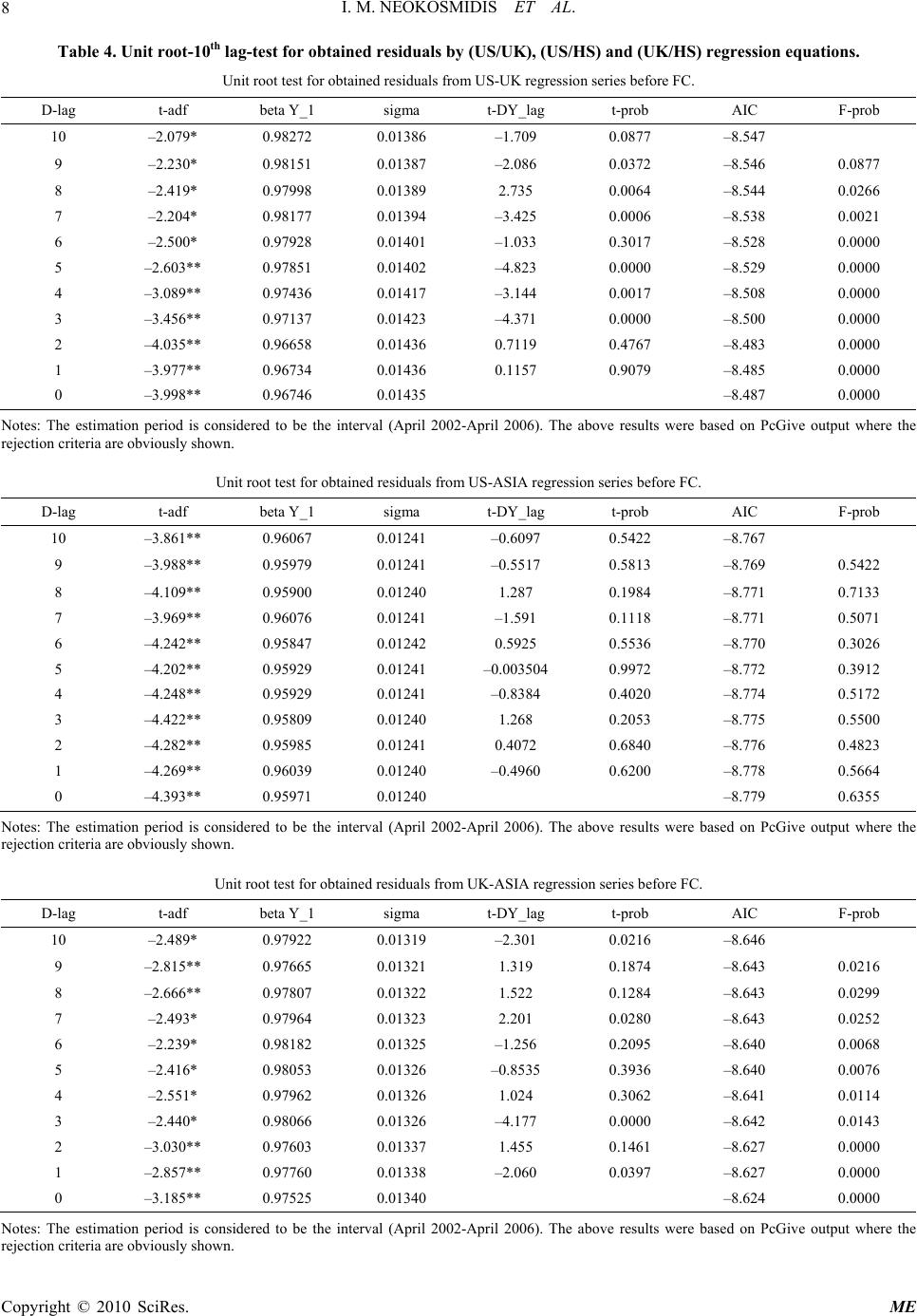





I. M. NEOKOSMIDIS ET AL. 8
y (US
om
t-DY_lag t-prob AIC F-prob
Table 4. Unit root-10th lag-test for obtained residuals b
Unit root test for obtained
/UK), (US/HS) and (UK/HS) regression equations.
US-UK regression series before FC. residuals fr
D-lag t-adf beta Y_1 sigma
10 –2.079* 0.98272 0.01386 –1.709 0.0877 –8.547
9 –2.230* 0.98151 0.01387 0.0877
6
7 –2.204* –8.538 0.0021
– 0–
0.0000
–2.086 0.0372 –8.546
8 –2.419* 0.97998 0.01389 2.735 0.0064 –8.544 0.026
0.98177 0.01394 –3.425 0.0006
6 2.500*0.97928 .01401 –1.033 0.3017 8.528 0.0000
5 –2.603** 0.97851 0.01402 –4.823 0.0000 –8.529
4 –3.089** 0.97436 0.01417 –3.144 0.0017 –8.508 0.0000
3 –3.456** 0.97137 0.01423 –4.371 0.0000 –8.500 0.0000
2 –4.035** 0.96658 0.01436 0.7119 0.4767 –8.483 0.0000
1 –3.977** 0.96734 0.01436 0.1157 0.9079 –8.485 0.0000
0 –3.998** 0.96746 0.01435 –8.487 0.0000
Notes: Tmationonsidered to be the interv002-Apr The abov were based on PcGive output where the
rejection criteria are obviously.
Unit roobtainedfrom US-gression sre FC.
D t-
he esti period is cal (April 2il 2006).e results
shown
ot test for residuals ASIA reeries befo
-lag t-adf beta Y_1 sigma DY_lagt-prob AIC F-prob
10 –3.861** 0.96067 0.01241 –0.7 0.52 60942–8.767
9 –3.988** 0.95979 0.01241 –0.5517 0.5813 –8.769 0.5422
8 –4.109** 0.95900 0.01240 1.287 0.1984 –8.771 0.7133
7 –3.969** –8.771 0.5071
–* 0–
– 0.3912
0.96076 0.01241 –1.591 0.1118
6 4.242*0.95847 .01242 0.5925 0.5536 8.770 0.3026
5 –4.202** 0.95929 0.01241 0.0035040.9972 –8.772
4 –4.248** 0.95929 0.01241 –0.8384 0.4020 –8.774 0.5172
3 –4.422** 0.95809 0.01240 1.268 0.2053 –8.775 0.5500
2 –4.282** 0.95985 0.01241 0.4072 0.6840 –8.776 0.4823
1 –4.269** 0.96039 0.01240 –0.4960 0.6200 –8.778 0.5664
0 –4.393** 0.95971 0.01240 –8.779 0.6355
Notes: Tmationonsidered to be the interv002-Aprhe abov were based on PcGive output where the
rejection criteria are obviously.
Unit roobtainedfrom UKgression sore FC.
D
he esti period is cal (April 2il 2006). Te results
shown
ot test for residuals -ASIA reeries bef
-lag t-adf beta Y_1 sigma t-DY_lag t-prob AIC F-prob
10 –2.489* 0.97922 0.01319 –2.1 0.06 3021–8.646
9 –2.815** 0.97665 0.01321 1.319 0.1874 –8.643 0.0216
8 –2.666** 0.97807 0.01322 1.522 0.1284 –8.643 0.0299
7 –2.493* –8.643 0.0252
– 0–
0.0076
0.97964 0.01323 2.201 0.0280
6 2.239*0.98182 .01325 –1.256 0.2095 8.640 0.0068
5 –2.416* 0.98053 0.01326 –0.8535 0.3936 –8.640
4 –2.551* 0.97962 0.01326 1.024 0.3062 –8.641 0.0114
3 –2.440* 0.98066 0.01326 –4.177 0.0000 –8.642 0.0143
2 –3.030** 0.97603 0.01337 1.455 0.1461 –8.627 0.0000
1 –2.857** 0.97760 0.01338 –2.060 0.0397 –8.627 0.0000
0 –3.185** 0.97525 0.01340 –8.624 0.0000
Notes: Tmation onsidered to be the interv002-Apri. The abov were based on PcGive output where the
rejection criteria are obviously.
he estiperiod is c
shown
al (April 2l 2006)e results

I. M. NEOKOSMIDIS ET AL.9
Unit robtained rom US-ion seriing FC.
D t-
ot test for oresiduals fUK regresses includ
-lag t-adf beta Y_1 sigma DY_lagt-prob AIC F-prob
10 –3.005** 0.97873 0.01646 –1.516 0.1297 –8.208
9 –3.123** 0.97795 0.01646 –1.2 0.05
–8.207 0.0726
–* 0–
0.0000
9946–8.208 0.1297
8 –3.278** 0.97690 0.01648 –0.8478 0.3967 –8.206 0.0438
7 –3.354** 0.97643 0.01648 –5.261 0.0000
6 3.804*0.97317 .01660 –3.494 0.0005 8.193 0.0000
5 –4.134** 0.97088 0.01665 –1.669 0.0954 –8.187
4 –4.313** 0.96975 0.01666 –0.7336 0.4633 –8.186 0.0000
3 –4.407** 0.96924 0.01666 –0.8469 0.3972 –8.187 0.0000
2 –4.517** 0.96864 0.01666 –4.029 0.0001 –8.188 0.0000
1 –4.991** 0.96542 0.01673 –9.822 0.0000 –8.180 0.0000
0 –6.328** 0.95547 0.01718 –8.127 0.0000
Notes: Tmationonsidered to be the interv002-Aprhe abov were based on PcGive output where the
rejection criteria are obviously.
oobtained rom US-Aession serding FC.
D t-
he esti period is c
shown
al (April 2il 2009). Te results
Unit rt test for oesiduals frSIA regries inclu
-lag t-adf beta Y_1 sigma DY_lagt-prob AIC F-prob
10 –3.372** 0.98750 0.01492 –0.9 0.81 17858–8.403
9 –3.378** 0.98748 0.01492 0.6637 0.5070 –8.404 0.8581
8 –3.365** 0.98754 0.01492 0.6143 0.5391 –8.405 0.7897
7 –3.351**–8.406 0.8376
–* 0–
0.5520
0.98759 0.01492 –1.759 0.0788
6 3.399*0.98741 .01492 –0.2129 0.8314 8.406 0.4147
5 –3.407** 0.98739 0.01492 –2.020 0.0435 –8.407
4 –3.459** 0.98719 0.01493 –2.055 0.0400 –8.405 0.2343
3 –3.527** 0.98694 0.01495 –0.7434 0.4573 –8.404 0.0922
2 –3.558** 0.98683 0.01495 –4.667 0.0000 –8.405 0.1183
1 –3.760** 0.98602 0.01503 –6.006 0.0000 –8.394 0.0001
0 –4.101** 0.98463 0.01519 –8.374 0.0000
Notes: Tmationonsidered to be the interv002-Apr The abov were based on PcGive output where the
rejectioniteria are obwn.
oottained rom UK-Aression seding FC.
D t-
he esti
cr
period is c
viously sho
al (April 2il 2009).e results
Unit r test for obesiduals frSIA regries inclu
-lag t-adf beta Y_1 sigma DY_lagt-prob AIC F-prob
10 –2.636** 0.98807 0.01538 –1.4 0.08 9550–8.343
9 –2.729** 0.98766 0.01540 0.2572 0.7971 –8.342 0.0508
8 –2.720** 0.98772 0.01539 1.151 0.2500 –8.343 0.1436
7 –2.666**–8.343 0.1574
–* 0–
0.0016
0.98798 0.01539 0.06629 0.9472
6 2.667*0.98799 .01539 –3.789 0.0002 8.344 0.2663
5 –2.886** 0.98698 0.01545 –3.279 0.0011 –8.337
4 –3.099** 0.98600 0.01549 2.248 0.0247 –8.332 0.0000
3 –2.960** 0.98664 0.01551 –6.017 0.0000 –8.330 0.0000
2 –3.406** 0.98452 0.01567 –2.834 0.0046 –8.311 0.0000
1 –3.641** 0.98348 0.01570 –4.886 0.0000 –8.307 0.0000
0 –4.102** 0.98135 0.01580 –8.295 0.0000
Notes: Tmationonsidered to be the interv002-Apri. The abov were based on PcGive output where the
rejectioniteria are obwn.
he esti
cr
period is c
viously sho
al (April 2l 2009)e results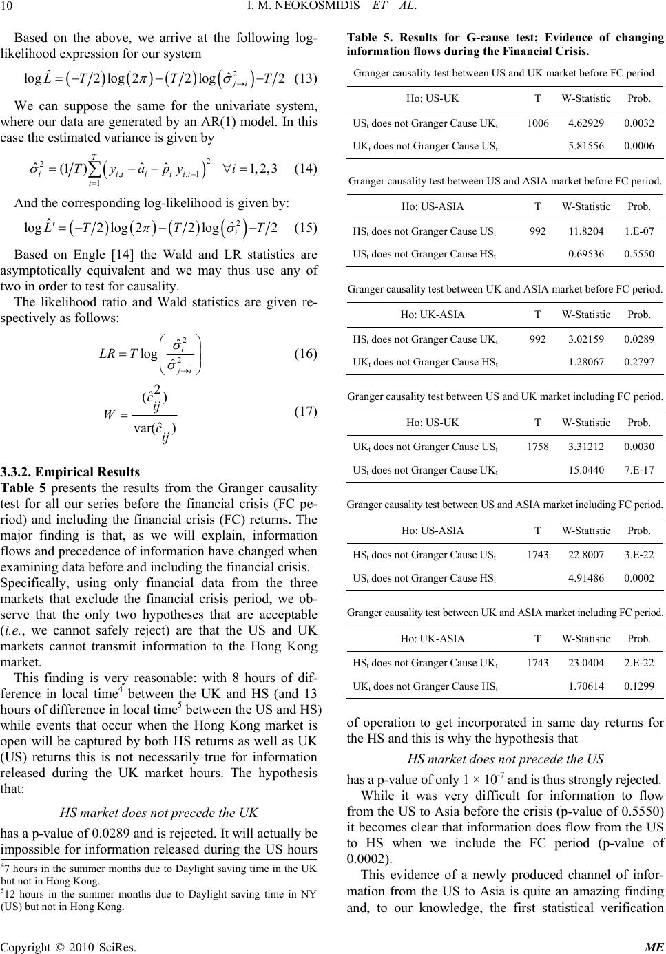

I. M. NEOKOSMIDIS ET AL. 10
Based on the a arrivfollow
likelihd expressir syste
bove, wee at the ing log-
ooon for oum




2
lo 22 ji
T TT


We can suppose the for tivariate syste,
ˆ
gLˆ log

log 2

2 (13)
e samhe unm
where our data are generated by an AR(1) model. In this
case the estimated variance is given by

2
2
,,1
ˆˆˆ
(1 )
T
iitiiit
Tyapy 



1t
(14) 1, 2, 3i
And the corresponding log-likelihood is given by:




2
ˆˆ
log2 log22log2
i
LTT T 
 (15)
Based on Engle [14] the Wald and LR statistics are
asymptotically equivalent and we ma thus use
two in order to test for causality.
re-
sp
yany of
The likelihood ratio and Wald statistics are given
ectively as follows:
2
2
logˆ
ˆi
j
i
LR T





(16)


)
ˆ
var(
)
2
ˆ
(c
ij
c
3.3.2. Empirical Results
Table 5 presents the results from the Granger causality
test for all our series before the financial crisis (FC pe-
riod) and including the financia
major finding is that, as we will explain, information
flows and precedence of information have changed when
xamining data before and including the financial crisis.
financial data from the three
uring the UK market hours. The hypothesis
th
Tults-cause tedence og
information flow the Financial Crisis.
y ten US andket beforeod.
Ho: US-UW-Statistb.
able 5. Res for Gst; Evif changin
s during
Granger causalitest betwe UK mar FC peri
K T icPro
USt does not Granger Cause UKt 1006 4.62929 0.0032
UKt does not Granger Cause USt 5.81556 0.0006
Granger causality test between US and ASIA market before FC period.
Prob. Ho: US-ASIA T W-Statistic
HSt does not Granger Cause USt 992 11.8204 1.E-07
USt does not Granger Cause HSt 0.69536 0.5550
G
Ho: UK-ASIA
ranger causality test between UK and ASIA market before FC period.
T W-StatisticProb.
HSt does not Granger Cause UKt 992 3.02159 0.0289
UKt does not Granger Cause HSt 1.28067 0.2797
Granger causality test between US and UK market including FC period.
ij
W (17)
Ho: US-UK T W-StatisticProb.
UKt does not Granger Cause USt 1758 3.31212 0.0030
USt does not Granger Cause UKt 15.0440 7.E-17
Granger causality test between US and ASIA market including FC period.
l crisis (FC) returns. The Ho: US-ASIA T W-StatisticProb.
HSt does not Granger Cause USt 1743 22.8007 3.E-22
USt does not Granger Cause HSt 4.914860.0002
e
Specifically, using only
markets that exclude the financial crisis period, we ob-
serve that the only two hypotheses that are acceptable
(i.e., we cannot safely reject) are that the US and UK
markets cannot transmit information to the Hong Kong
market.
This finding is very reasonable: with 8 hours of dif-
Granger causality test between UK and ASIA market including FC period.
Ho: UK-ASIA T W-StatisticProb.
HSt does not Granger Cause UKt 1743 23.0404 2.E-22
UKt does not Granger Cause HSt 1.70614 0.1299
ference in local time4 between the UK and HS (and 13
hours of difference in local time5 between the US and HS)
while events that occur when the Hong Kong market is
open will be captured by both HS returns as well as UK
(US) returns this is not necessarily true for information
released d
of operation to get incorporated in same day returns for
the HS ane hypoth
HS market does not precede the US
h ands r.
ult for inf
om the US to Asia before the crisis (p-value of 0.5550)
to HS when we include the FC period (p-value of
0.0002).
prd o-
mation from the US to Asia is quite an amazing finding
and, to our knowledge, the first statistical verification
d this is why thesis that
as a p-value of only 1 × 10-7 is thu stronglyejected
While it was very difficormation to flow
at:
HS market does not precede the UK
has a p-value of 0.0289 and is rejected. It will actually be
impossible for information released during the US hours
fr
it becomes clear that information does flow from the US
This evidence of a newlyoducechannelf infor
47 hours in the summer months due to Daylight saving time in the UK
but not in Hong Kong.
512 hours in the summer months due to Daylight saving time in NY
(US) but not in Hong Kong.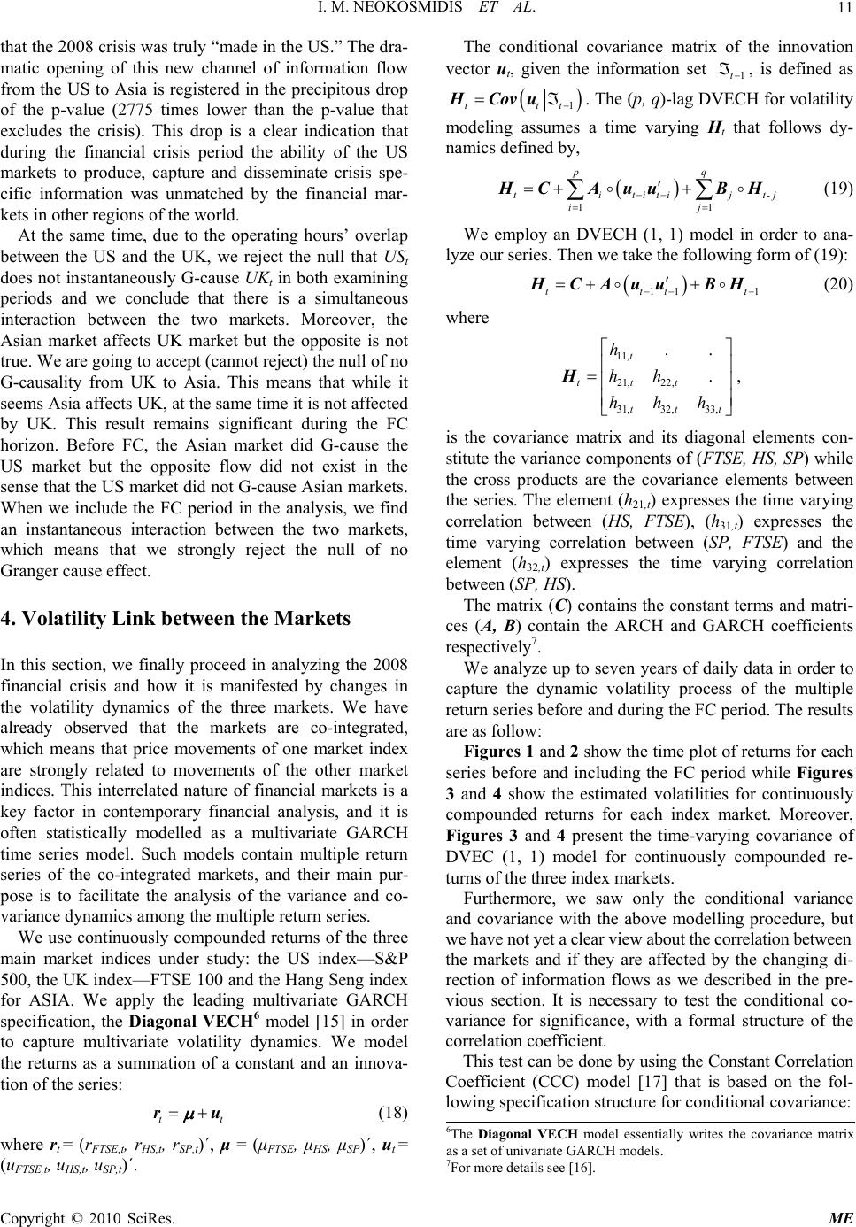

I. M. NEOKOSMIDIS ET AL.11
tmade in t T
atic opening of this new channel of information flow
ation that
during thef the US
ci
antaneously G-cause UK in both examining
pe
een the two markets,
w
e analysis of the variance and co-
s.
e three
ain market indices under study: the US index—S&P
hat the 2008 crisis was truly “he US.”he dra-
m
from the US to Asia is registered in the precipitous drop
of the p-value (2775 times lower than the p-value that
excludes the crisis). This drop is a clear indic
financial crisis period the ability o
markets to produce, capture and disseminate crisis spe-
fic information was unmatched by the financial mar-
kets in other regions of the world.
At the same time, due to the operating hours’ overlap
between the US and the UK, we reject the null that US t
does not instt
riods and we conclude that there is a simultaneous
interaction between the two markets. Moreover, the
Asian market affects UK market but the opposite is not
true. We are going to accept (cannot reject) the null of no
G-causality from UK to Asia. This means that while it
seems Asia affects UK, at the same time it is not affected
by UK. This result remains significant during the FC
horizon. Before FC, the Asian market did G-cause the
US market but the opposite flow did not exist in the
sense that the US market did not G-cause Asian markets.
When we include the FC period in the analysis, we find
an instantaneous interaction betw
hich means that we strongly reject the null of no
Granger cause effect.
4. Volatility Link between the Markets
In this section, we finally proceed in analyzing the 2008
financial crisis and how it is manifested by changes in
the volatility dynamics of the three markets. We have
already observed that the markets are co-integrated,
which means that price movements of one market index
are strongly related to movements of the other market
indices. This interrelated nature of financial markets is a
key factor in contemporary financial analysis, and it is
often statistically modelled as a multivariate GARCH
time series model. Such models contain multiple return
series of the co-integrated markets, and their main pur-
ose is to facilitate thp
variance dynamics among the multiple return serie
We use continuously compounded returns of th
m
500, the UK index—FTSE 100 and the Hang Seng index
for ASIA. We apply the leading multivariate GARCH
specification, the Diagonal VECH6 model [15] in order
to capture multivariate volatility dynamics. We model
the returns as a summation of a constant and an innova-
tion of the series:
tt
ru

(18)
where rt = (rFTSE,t, rHS,t, rSP,t)΄, μ = (μFTSE, μHS, μSP)΄, ut =
(uFTSE,t, uHS,t, uSP,t)΄.
The conditional covariance matrix of the innovation
vector ut, given the information set 1t
, is defined as


H1ttt Covu . The (p, q)-lag DVECH for volatility
modeling assumes a time varying Ht that follows dy-
namics defined by,

11
pq
tititijt-j
ij



 


H
CAuu BH (19)
We employ an DVECH (1, 1) model in order to ana-
lyze our series. Then we take the following form of (19):


1 1t1ttt


 
H
CAuu BH (20)
where
11,
21, 22,
31, 32, 33,
..
.
t
ttt
ttt
h
hh
hhh











H
is the covariance matrix and its diagonal elements con-
stitute the variance co
,
mponents of (FTSE, HS, SP) while
the cross products are the covariance elements between
the series. The element (h21,t) expresses the tim
correlation between (HS, FTSE), (h31,t) expresses the
tim
between (SP, HS).
The matrix (C) contains the constant term
) contain the ARCH and GARCH coefficients
respectively7.
We analyze up to seven years of daily data in order to
capture the dynamic volatility processf the multiple
return series before and during the FC period. The results
are as follow:
saw only the conditional variance
an
d if they are affected by the changing di-
re
icient.
e varying
e varying correlation between (SP, FTSE) and the
element (h32,t) expresses the time varying correlation
s and matri-
ces (A, B
o
Figures 1 and 2 show the time plot of returns for each
series before and including the FC period while Figures
3 and 4 show the estimated volatilities for continuously
compounded returns for each index market. Moreover,
Figures 3 and 4 present the time-varying covariance of
DVEC (1, 1) model for continuously compounded re-
turns of the three index markets.
Furthermore, we
d covariance with the above modelling procedure, but
we have not yet a clear view about the correlation between
the markets an
ction of information flows as we described in the pre-
vious section. It is necessary to test the conditional co-
variance for significance, with a formal structure of the
correlation coeff
This test can be done by using the Constant Correlation
Coefficient (CCC) model [17] that is based on the fol-
lowing specification structure for conditional covariance:
6The Diagonal VECH model essentially writes the covariance matrix
as a set of univariate GARCH models.
7For more details see [16].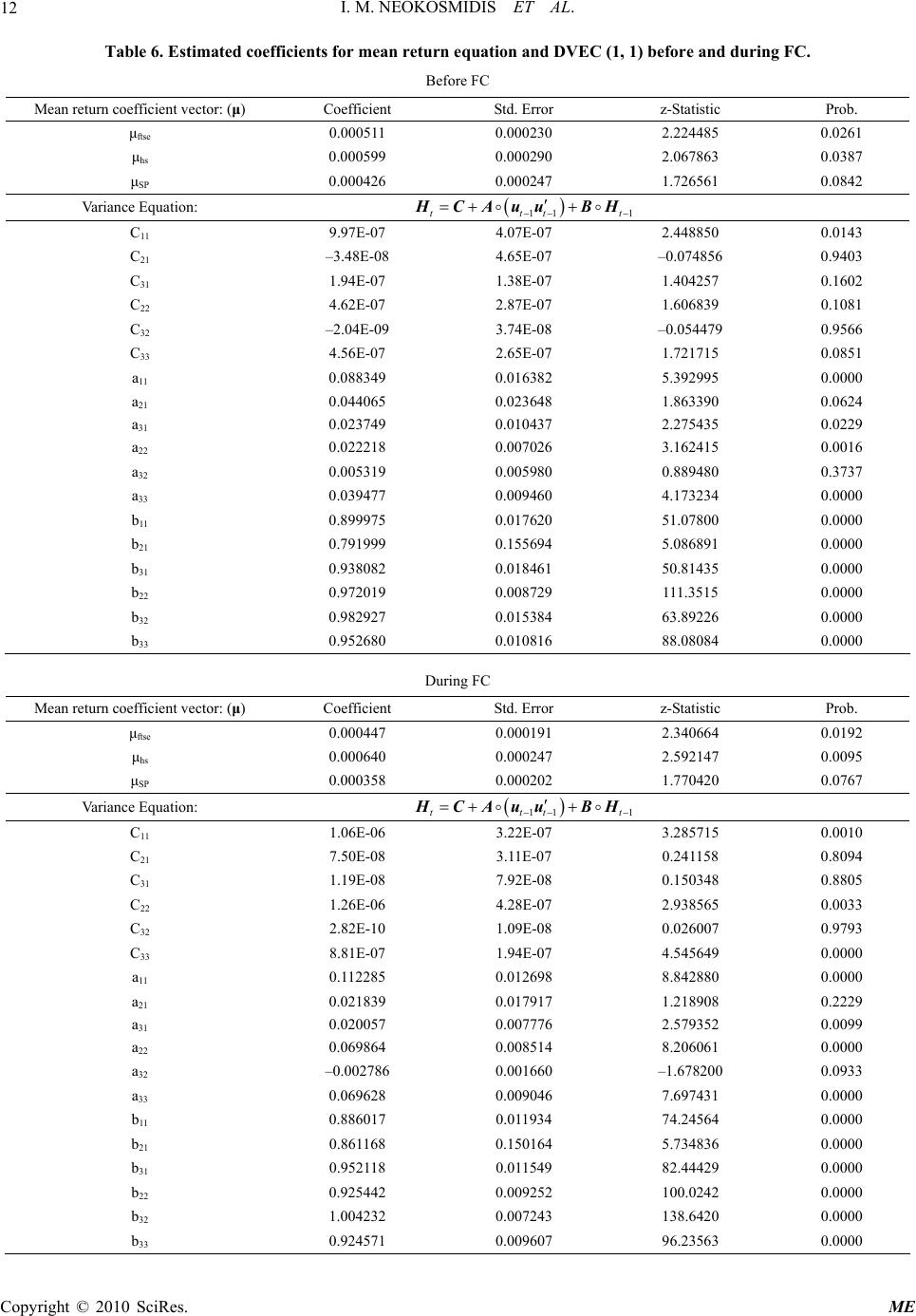

I. M. NEOKOSMIDIS ET AL. 12
equ
ore F
Table 6. Estimated coefficients for mean return
Bef
Mean return coefficient vector: (μ) Coefficient
ation and DVEC (1, 1) before and during FC.
C
Std. Error z-Statistic Prob.
μftse 0.000511 0.000230 2.224485 0.0261
μhs 0.000599
μSP 0.000426
0.000290 2.067863 0.0387
0.000247 1.726561 0.0842
Variance Equation:


11 1tttt


Auu BH

HC
C11 9.97E-07 4.07E-07 2.448850 0.0143
C21 –3.48E-08 4.65E-07 –0.074856 0.9403
0.
22
–0.
0.044065 0.023648 1.863390 0.0624
C31 1.94E-07 1.38E-07 1.404257 1602
C4.62E-07 2.87E-07 1.606839 0.1081
C32 –2.04E-09 3.74E-08 054479 0.9566
C33 4.56E-07 2.
0.088349 0.
65E-07
016382 5.
1.721715
392995
0.0851
0.0000 a11
a21
a31
a22
0.023749 0.010437 2.275435 0.0229
0.022218 0.007026 3.162415 0.0016
a32 0.005319 0.005980 0.889480 0.3737
a33
b11
0.039477 0.009460 4.173234 0.0000
0.899975 0.017620 51.07800 0.0000
b21 0.791999 0.155694 5.086891 0.0000
b31 0.938082 0.018461 50.81435 0.0000
b22 0.972019 0.008729 111.3515 0.0000
b32 0.982927 0.015384 63.89226 0.0000
b33 0.952680 0.010816 88.08084 0.0000
During FC
Mean return coμ) efficient vector: (Coefficient Std. Error z-Statistic Prob.
μftse 0.000447 0.000191 2.340664 0.0192
μhs 0.000640 0.000247 2.592147 0.0095
μSP 0.000358 0.000202 1.770420 0.0767
Variancuation: e Eq


11 1tttt



uu   HCA BH
C11 1.06E-06 3.22E-07 3.285715 0.0010
C21 7.50E-08 3.11E-07 0.241158 0.8094
0.
22
C31 1.19E-08 7.92E-08 0.150348 8805
C1.26E-06 4.28E-07 2.938565 0.0033
C32 2.82E-10 1.09E-08 0.026007 0.9793
C33 8.81E-07 1.
0.112285 0.
94E-07
012698
4.545649
8.842880
0.0000
0.0000 a11
a21
a
0.021839 0.
0.020057
017917 1.
0.007776
218908
2.579352
0.2229
0.0099
31
a22 0.069864 0.008514 8.206061 0.0000
a32
a
–0.002786 0.001660 –1.678200 0.0933
33
b11
0.069628 0.009046 7.697431 0.0000
0.886017 0.011934 74.24564 0.0000
b21 0.861168 0.150164 5.734836 0.0000
b31 0.952118 0.011549 82.44429 0.0000
b22 0.925442 0.009252 100.0242 0.0000
b32 1.004232 0.007243 138.6420 0.0000
b33 0.924571 0.009607 96.23563 0.0000

I. M. NEOKOSMIDIS ET AL.13
-.0 6
-.0 4
-.0 2
.00
.02
.04
.06
20022003 2004 2005
RETURNS_FTSE 100
-.0 6
-.0 4
-.0 2
.00
.02
.04
.06
20022003 2004 2005
RETURNS_HS
-.0 6
-.0 4
-.0 2
.00
.02
.04
.06
20022003 2004 2005
RETURNS_S&P 500
-.1 0 0
-.0 7 5
-.0 5 0
-.0 2 5
.000
.025
.050
.075
.100
Figure 1. Continuously compounded returns of FTSE 100,
S&P 500 and Hang Seng time series before FC period.
20022003 2004 2005 2006 2007 2008
RETSE 100 TURNS_F
-. 1 5
-. 1 0
-. 0 5
.15
.00
.05
.10
20022003 2004 2005 2006 2007 2008
RETURNS_HS
-. 1 2
-. 0 8
-. 0 4
.00
.04
.08
.12
20022003 2004 2005 20062007 2008
RETURNS_S&P 500
Figure 2. Continuously compounded returns of FTSE 100,
S&P 500 and Hang Seng time series during FC period.

I. M. NEOKOSMIDIS ET AL. 14
.0000
.0002
.0004
.0006
.0008
.0010
20022003 20042005
Var(RETURNS_FTSE 100)
-.00004
.00000
.00004
.00008
.00012
20022003 20042005
Cov(RETURNS_FTSE 100, RETURNS_HS)
.00004
.00008
.00012
.00016
.00020
.00024
20022003 20042005
Var(RETURNS_HS)
-.00005
.000 00
.000 05
.000 10
.000 15
.000 20
20022003 2004 2005
Cov(RETURNS_FTSE 100, RETURNS_S&P 500)
-.00001
.00000
.00001
.0006
.00002
.00003
.00004
.00005
20022003 2004 2005
Cov(RETURNS_HS, RETURNS_S&P 500)
.0000
.0001
.0002
.0003
.0004
.0005
200220032004 2005
Var(RETURNS_S&P 500)
Figure 3. Conditional variance-covariance representation of estimated return series before FC time period.
.0000
.0005
.0010
.0015
.0020
.0025
.0030
20022003 2004 2005 2006 2007 2008
Var(RETURNS_FTSE 100)
-.00010
-.00005
.00000
.00005
.00010
.00015
.00020
20022003 2004 2005 2006 2007 2008
Cov(RETURNS_FTSE 100, RETURNS_HS)
.000
.001
.002
.003
.004
.005
20022003 2004 2005 2006 2007 2008
Var(RET URNS_HS)
-.0002
-.0001
.0000
.0001
.0002
20022003 2004 2005 2006 2007 2008
Cov(RETURNS_FTSE 100, RETURNS_S&P 500)
-.00006
-.00004
-.00002
.0030
.00000
.00002
.00004
20022003 2004 2005 2006 2007 2008
Cov(RETURNS_HS, RETURNS_S&P 500)
.0000
.0005
.0010
.0015
.0020
.0025
20022003 2004 2005 20062007 2008
Var(RETURNS_S&P 500)
Figure 4. Conditional variance-covariance representation of estimated return series during FC time period.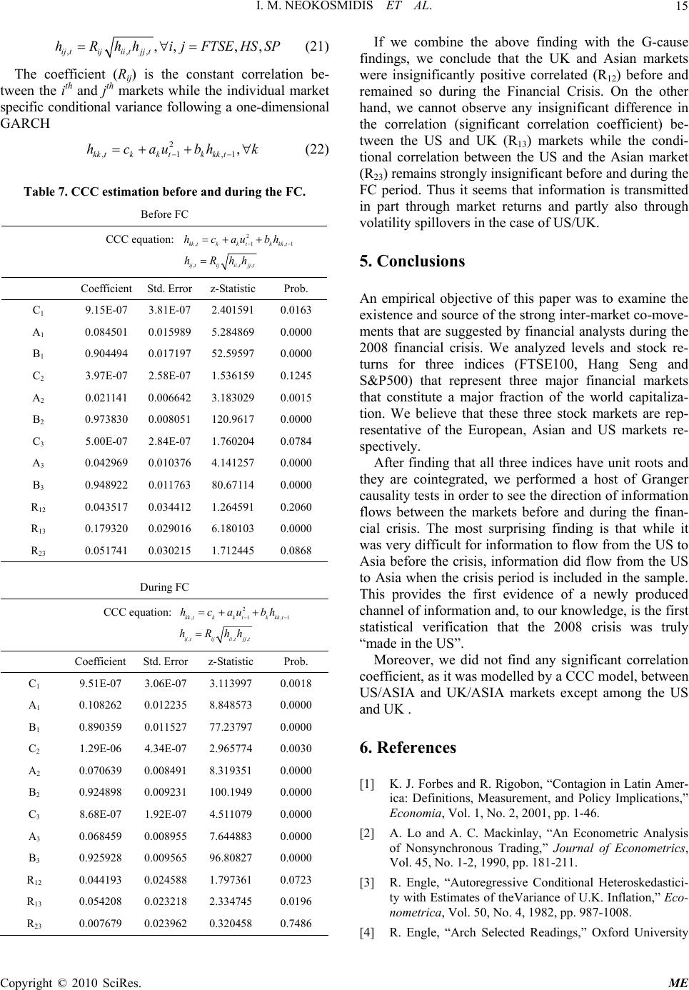

I. M. NEOKOSMIDIS ET AL.15
,,,
,,, ,
ij tijii tjj t
hRhh ijFTSEHSS If we combine the above finding with the G-cause
findings, we conclude that the UK and Asian markets
were insignificantly positive correlated (R12) before and
remained so during the Financial Crisis. On the other
hand, we cannot observe any insignificant difference in
the correlation (significant correlation coefficient) be-
tween the US and UK (R13) markets while the condi-
tional correlation between the US and the Asian market
(R23) remains strongly insignificant before and during the
FC period. Thus it seems that information is transmitted
in part through market returns and partly also through
volatility spillovers in the case of US/UK.
5. Conclusions
An empirical objective of this paper was to examine the
existence and source of the strong inter-market co-move-
ments that are suggested by financial analysts during the
2008 financial crisis. We analyzed levels and stock re-
turns for three indices (FTSE100, Hang Seng and
S&P500) that represent three major financial markets
that constitute a major fraction of the world capitaliza-
tion. We believe that these three stock markets are rep-
resentative of the European, Asian and US markets re-
spectively.
After finding that all three indices have unit roots and
nger
causality tests toirinfn
flows betweenrkets bh-
cial s. Thurinatit
was diffinfo tto
Asia fore the crisis, in dromS
to Asia when the crisis peri is included in the sample.
This provides the first ef a newly produced
channel of information knowledge, is the first
statistical verifice 2008 crisis was truly
“made in the US”.
Moreover, we did noany significanrrelation
coefficient, ao ael, en
US/AIA eongS
and UK .
6. Rren
[1] J. For. RCo Latin Amer-
: Defineas and plications,”
nomi Nopp
[2] Lo anaAntricis
Nonsys TJournal of Econs,
, No. 1-2, 1990, pp. 181-211.
[3] itionaeroskedastici-
ith Ete flato-
metric , N, pp. 987-1008.
[4] R. Engle, “Arch Selected Readings,” Oxford University
P (21)
The coefficient (Rij) is the constant correlation be-
tween the ith and jth markets while the individual market
specific conditional variance following a one-dimensional
GARCH
1
k (22)
Table 7. CCC estimation before and during the FC.
Before FC
CCC equation: ,1
2
,1,
,
kk tkktkkk t
hcaubh

 
2
,1 kk tkktkkk t
hcaubh

 
,, ij tijii tjjt hRhh
,
Coefficient Std. Error z-Statistic Prob.
C1 9.15E-07 3.81E-07 2.401591 0.0163
A1 0.084501 0.015989 5.284869 0.0000
B1 0.904494 0.017197 52.59597 0.0000
C2 3.97E-07 2.58E-07 1.536159 0.1245
A2 0.021141 0.006642 3.183029 0.0015
B2 0.973830 0.008051 120.9617 0.0000
C3 5.00E-07 2.84E-07 1.760204 0.0784
A3 0.042969 0.010376 4.141257 0.0000
R12 0.043517 0.034412 1.264591
B3 0.948922 0.011763 80.67114 0.0000
0.2060
R13 0.179320 0.029016 6.180103 0.0000
R23 0.051741 0.030215 1.712445 0.0868
During FC
CCC equation:
2
,1 kk tkktkkk t
hcaub

 ,1 h
,,,ij tijii tjj t
hRhh
Coefficient z-StStd. Error atistic Prob.
C1 9.51E-07 3.06E97 0.0018 -07 3.1139
A0.10825 8.848573 0.0000
B1 0.890359 7 77.23797 0.0000
C
0.
0.
8
0.
0.
R0.
R0.
R0.
1 62 0.30122
0.01152
2 1.29E-06 4.34E-07 2.965774 0.0030
A2 070639 0.008491 8.319351 0.0000
B2 924898 0.009231 100.1949 0.0000
C3 .68E-07 1.92E-07 4.511079 0.0000
A3 068459 0.008955 7.644883 0.0000
B3 925928 0.009565 96.80827 0.0000
12 044193 0.024588 1.797361 0.0723
13 054208 0.023218 2.334745 0.0196
23 007679 0.023962 0.320458 0.7486
they are cointegrated, we performed a host of Gra
in order see the dection of ormatio
the ma
e most s
efore a
prising f
nd during t
ding is th
e finan
while crisi
verycult for irmation to flow fromhe US
beformationid flow f the U
od
vidence o
and, to our
ation that th
t find t co
s it was mdelled by CCC modbetwe
SIA and UK/AS marketsxcept am the U
efeces
K.bes and Rigobon, “ntagion in
ica
Eco
itions, M
a, Vol. 1,
urement,
. 2, 2001,
Policy Im
. 1-46.
A. d A. C. Mckinlay, “ Econome Analys
of
Vol. 45
nchronourading,” ometric
R. Engle, “Autoregressive Condl Het
ty wstimates of heVariancof U.K. Inion,” Ec
no a, Vol. 50o. 4, 1982

I. M. NEOKOSMIDIS ET AL. 16
ss, Ox5.
[5]
d W. A. Fuller, “Likelihood Ratio Statis-
ressive Time Series with a Unit Root,”
Econometrica, Vol. 49, No. 4, 1981, pp. 1057-1072.
“Cointegration and
metrics,”
elihood Ratio and Lagrange Multi-
al Economy, Vol. 96, No. 1,
Preford, 199
R. Engle, “The use of ARCH/GARCH Models in Applied
Econometrics,” Journal of Economic Perspectives, Vol.
15, No. 4, 2001, pp. 157-168.
[6] T. Bollerslev, “Generalized Autoregressive Conditional
Heteroscedasticity,” Journal of Econometrics, Vol. 31,
No. 3, 1986, pp. 307-327.
[7] T. Bollerslev, R. F. Engle and D. B. Nelson, “ARCH
Models,” In: R. Engle and D. McFadden, Eds., Handbook
of Econometrics, North Holland Press, Amsterdam, 1994.
[8] D. A. Dickey and W. A. Fuller, “Distributions of the
Estimators for Autoregressive Time Series with a Unit
Root,” Journal of American Statistical Association, Vol.
74, No. 366, 1979, pp. 427-481.
[9] D. A. Dickey an
tics for Autoreg
198
[10] H. Akaike, “Information Theory and an Extension of the
Maximum Likelihood Principle,” In: B. N. Petrov and
Csaki, Eds., 2nd International Symposium on Information
Theory, Academia Kiado, Budapest, 1973, pp. 267-281.
[11] R. Harris and R. Sollis, “Applied Time Series Modelling
and Forecasting,” John Wiley, New York, 2003.
[12] R. F. Engle and C. W. J. Granger,
Error Correction: Representation, Estimation and Test-
ing,” Econometrica, Vol. 55, No. 2, 1987, pp. 251-276.
[13] C. Gourieroux and J. Jasiak, “Financial Econo
Princeton University Press, Princeton and Oxford, 2001.
[14] R. Engle, “Wald, Lik
plier Tests in Econometrics,” In: Z. Griliches and M. D.
lntriligator, Eds., Handbook of Econometrics II, 1983, pp.
796-801.
[15] T. Bollerslev, R. Engle and J. M. Wooldridge, “A Capi-
tal-Asset Pricing Model with Time-Varying Covari-
ances,” Journal of politic
8, pp. 116-131.
[16] R. Tsay, “Analysis of Financial Time Series,” John Wiley
& Sons, New Jersey, 2005.
[17] T. Bollerslev, “Modeling the Coherence in Short-Term
Nominal Exchange Rates: A Multivariate Generalized
ARCH Approach,” Review of Economics and Statistics,
1990.