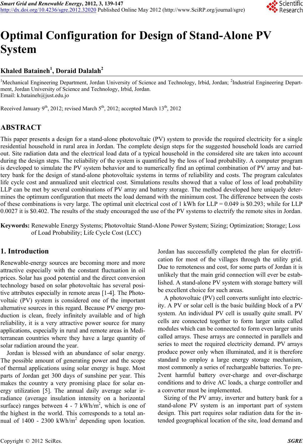
Smart Grid and Renewable Energy, 2012, 3, 139-147
http://dx.doi.org/10.4236/sgre.2012.32020 Published Online May 2012 (http://www.SciRP.org/journal/sgre) 1
Optimal Configuration for Design of S tand-Alone PV
System
Khaled Bataineh1, Doraid Dalalah2
1Mechanical Engineering Department, Jordan University of Science and Technology, Irbid, Jordan; 2Industrial Engineering Depart-
ment, Jordan University of Science and Technology, Irbid, Jordan.
Received January 9th, 2012; revised March 5th, 2012; accepted March 13th, 2012
ABSTRACT
This paper presents a design for a stand-alone photovoltaic (PV) system to provide the required electricity for a single
residential household in rural area in Jordan. The complete design steps for the suggested household loads are carried
out. Site radiation data and the electrical load data of a typical household in the considered site are taken into account
during the design steps. The reliability o f the system is quantified by the loss of load probability. A computer program
is developed to simulate the PV system behavior and to numerically find an optimal combination of PV array and bat-
tery bank for the design of stand-alone photovoltaic systems in terms of reliability and costs. The program calculates
life cycle cost and annualized unit electrical cost. Simulations results showed that a value of loss of load probability
LLP can be met by several combinations of PV array and battery storage. The method developed here uniquely deter-
mines the optimum configuration that meets the load demand with the mini mum c os t. Th e difference between the costs
of these combinations is v ery large. The optimal unit electrical cost of 1 kWh for LLP = 0.049 is $0.293 ; while for LLP
0.0027 it is $0.402. Th e results of the study encouraged the use of the PV systems to electrify the remote sites in Jordan.
Keywords: Renewable Energy Systems; Photovoltaic Stand-Alone Power System; Sizing; Optimization; Storage; Loss
of Load Probability; Life Cycle Cost (LCC)
1. Introduction
Renewable-energy sources are becoming more and more
attractive especially with the constant fluctuation in oil
prices. Solar has good po tential and the d irect conversion
technology based on solar photovoltaic has several posi-
tive attr ibutes especial ly in remote areas [1-4]. The Photo-
voltaic (PV) system is considered one of the important
alternative sources in this regard. Because PV energy pro-
duction is clean, freely infinitely available and of high
reliability, it is a very attractive power source for many
applications, especially in rural and re mote areas in Medi-
terranean countries where they have a large quantity of
solar radiation around the year.
Jordan is blessed with an abundance of solar energy.
The possible amount of generating power and the scope
of thermal applications using solar energy is huge. Most
parts of Jordan get 300 days of sunshine per year. This
makes the country a very promising place for solar en-
ergy utilization [5]. The annual daily average solar ir-
radiance (average insulation intensity on a horizontal
surface) ranges between 4 - 7 kWh/m2, which is one of
the highest in the world. This corresponds to a total an-
nual of 1400 - 2300 kWh/m2 depending upon location.
Jordan has successfully completed the plan for electrifi-
cation for most of the villages through the utility grid.
Due to remoteness and cost, for some parts of Jordan it is
unlikely that the main grid connection will ever be estab-
lished. A stand-alone PV system with storage battery will
be excellent choice for such areas.
A photovoltaic (PV) cell converts su nlig h t into electri c-
ity. A PV or solar cell is the b asic building block of a PV
system. An individual PV cell is usually quite small. PV
cells are connected together to form larger units called
modules which can be connect ed t o form even larger units
called arrays. These arrays are connected in parallels and
series to meet the required electricity demand. PV arrays
produce power only when illuminated, and it is therefore
standard to employ a large energy storage mechanism,
most commonly a series of rechargeable batteries. To pre-
2vent harmful battery over-charge and over-discharge
condition s and to drive AC loads, a charge controller and
a converter m ust be implemented.
Sizing of the PV array, inverter and battery bank for a
stand-alone PV system is an important part of system
design. This part requires solar radiation data for the in-
tended geographical location of the site, load demand and

Optimal Configuration for Design of Stand-Alone PV System
140
manufacturing data for PV modules, inverters and bat-
teries and their operational efficiencies. Numerous stud-
ies have been conducted to develop a sizing method
which is both easy to apply and highly reliable [6]. Most
of these methods assume constant system load and con-
trol the variables that have an influence on the degree of
reliability. Methods that are based on the concept of
power supply during a number of autonomous days are
typically used. These methods are simple and assure the
required reliability of the PV system during autonomous
days. In these methods, the storage system meets the load
demand. The storage system capacity is regarded as a
measure of reliability of the PV system. So the reliability
is determined by the autonomous days. These methods
exhibit no direct relationship between the PV array out-
put and the storage system capacity. Also, the resultant
sizing of the combination of PV array and battery bank
for a solar PV system is not necessarily optimal. Method
based on the study and characterization of daily energy
balances is developed [7,8]. More universal results are
obtained when implementing these methods. Another
method design of a stand-alone PV system is based on
the concep t of reliability of the power supply to the load ,
which is usually quantified by the loss of power supply
probability (LPSP) [9-17]. This concept is defined as the
relationship between the energy deficit and the energy
demand during the total operation time of the installation.
In statistical terms, the LLP value refers to the probabil-
ity that the system will be unable to meet energy demand.
Due to the random nature of the energy source, great
effort must be made to optimize the design of stand-alone
photovoltaic systems in terms of both energy consump-
tion and costs. The cost of RE generation plays a major
role in determining the effectiveness of the RE systems.
Hernández et al. examined the development of the four
main renewable energy technologies (RET) in Spain in
the latest years: biomass, small hydro (SH), solar photo-
voltaic (solar PV) and wind [18]. The study concluded
that Spain is suitab le in meeting the RE generation target
but not efficient in costs. The task of sizing should com-
promise between cost and reliability. Accurate sizing
ensures that demand is met and allows costs to be cut in
the future. This will allow a practical use of these sys-
tems in the renewable energies market. Sizing a PV sys-
tem means determining both the number and area of
modules to install and the capacity or total number of
ampere-hours collectable in the battery.
In this work a standard model based on daily energy
balance is used to determine system size. Several design
criteria are investigated. Numerical methods based on de-
tailed simulations of PV system behavior which are per-
formed over a specific period of time are used. The energy
balance of the PV system and the state of charge of the
battery are calculated daily. The simulation period is taken
to be one year to have statistical significance of the value
of loss of load probabilities LLP. A computer program is
developed to simulate the PV system behavior and to nu-
merically find an optimal combination of PV array and
battery bank for the design of stand-alone photovoltaic
systems in terms of reliability and costs. The detailed de-
sign and economical analysis of a stand-alone PV system
to provide the required electrical energy for a single resi-
dential household in Jordan is presented. The considered
location is Jordan University of Science and Technology,
which is located in t he northern part of Jordan.
2. Ease the Household PV System
Configuration
The basic configuration of a PV stand-alone system shown
in Figure 1 is considered in this study. The system con-
sists mainly of solar panels, inverter, batteries and load.
The function of the PV array is to convert the sunlight
directly into DC electrical power. The inverter is used to
convert the DC electrical power into AC power; to match
the requirements of the common household AC appliances.
The excessive part of DC power is stored in the b attery to
be used when there is no sunshine. The controller m onit ors
the electrical input from the solar panels and controls the
amount going directly into the inverter and the amount for
charging and discharging of the battery bank.
3. Prepare Site Meteorological Data
To predict the performance of a PV system in a location,
it is necessary to collect the meteorological or environ-
mental data for the site location under consideration. The
monthly average daily solar radiation data incident on a
horizontal surface at the considered site is shown in Fig-
ure 2. It is clear from Figure 2 that solar energy incident
in the considered site is very high especially during the
summer months, where it exceeds 7 kWh/m2/day on hori-
zontal. Table 1 lists the average number of clear days for
each month and the average number of shining hours for
each month. It is clear from Table 1 that even in winter,
Jordan enjoys more than twenty days of sunshine per
month. The total number of sunshine days in Jordan ex-
ceeds 300 annually.
Figure 1. Schematic of stand-alone PV system.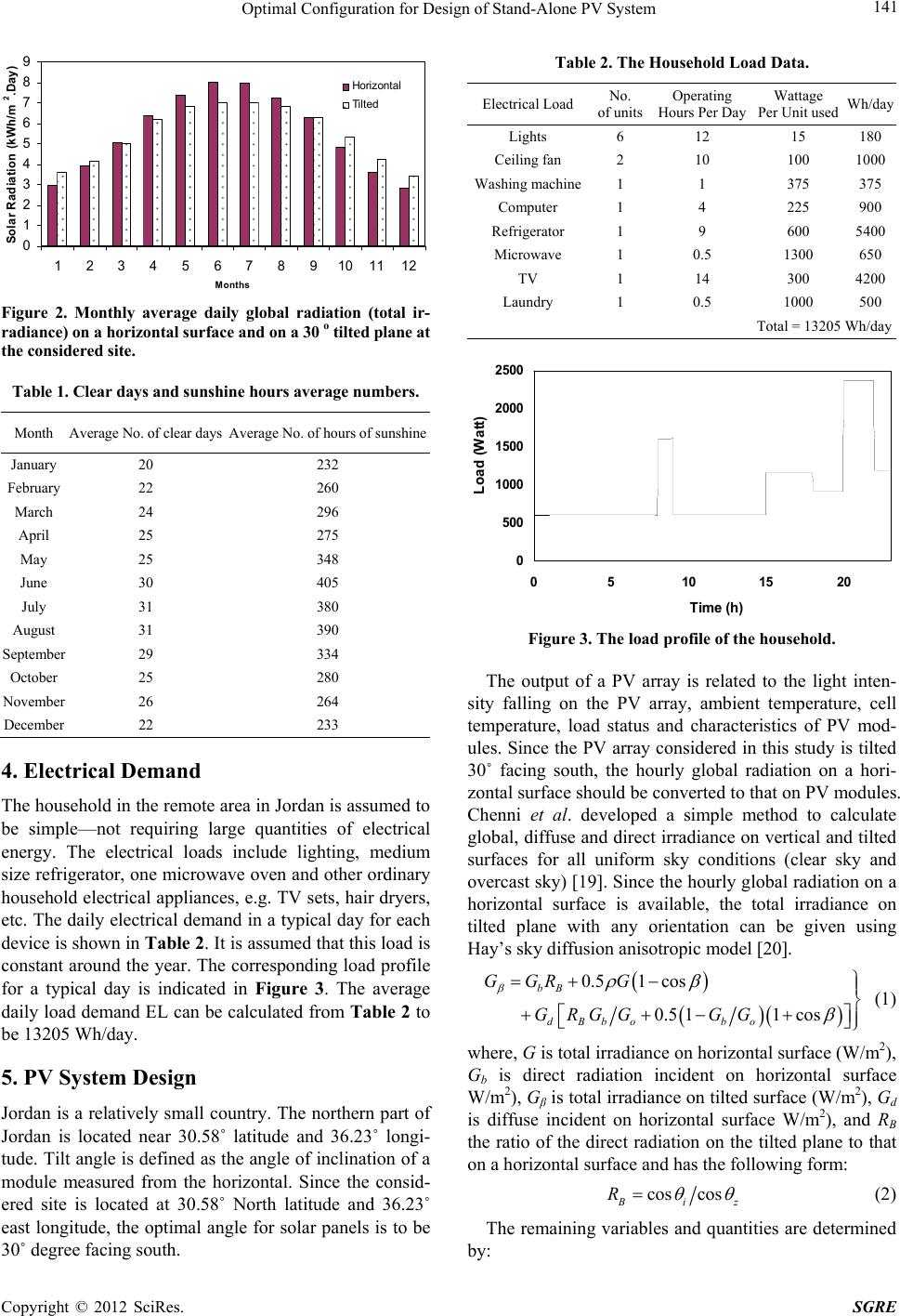

Optimal Configuration for Design of Stand-Alone PV System 141
0
1
2
3
4
5
6
7
8
9
123456789101112
M onths
Solar Radiat ion (kWh/m
2
.Day)
Horizontal
T ilted
Figure 2. Monthly average daily global radiation (total ir-
radiance) on a horizontal surface and on a 30 o tilted plane at
the considered site.
Table 1. Clear days and sunshine hours average numbers.
Month Average No. of clear daysAverage No. of hours of sunshine
January 20 232
February 22 260
March 24 296
April 25 275
May 25 348
June 30 405
July 31 380
August 31 390
September 29 334
October 25 280
November 26 264
December 22 233
4. Electrical Demand
The household in the remote area in Jordan is assumed to
be simple—not requiring large quantities of electrical
energy. The electrical loads include lighting, medium
size refrigerator, one microwave oven and other ordinary
household electrical appliances, e.g. TV sets, hair dryers,
etc. The daily electrical demand in a typical day for each
device is shown in Table 2. It is assumed that this load is
constant around the year. The corresponding load profile
for a typical day is indicated in Figure 3. The average
daily load demand EL can be calculated from Table 2 to
be 13205 Wh/day.
5. PV System Design
Jordan is a relatively small coun try. The northern part of
Jordan is located near 30.58˚ latitude and 36.23˚ longi-
tude. Tilt angle is defined as the angle of inclination of a
module measured from the horizontal. Since the consid-
ered site is located at 30.58˚ North latitude and 36.23˚
east longitude, the optimal angle for solar panels is to be
30˚ degree f a cing south.
Table 2. The Household Load Data.
Wh/day
Wattage
Per Unit used
Operating
Hours Per Day
No.
of units
Electrical Load
180 15 12 6 Lights
1000100 10 2 Ceiling fan
375 375 1 1 Washing machine
900 225 4 1 Computer
5400600 9 1 Refrigerator
650 1300 0.5 1 Microwave
4200300 14 1 TV
500 1000 0.5 1 Laundry
Total = 13205 Wh/day
0
500
1000
1500
2000
2500
0510 1520
Ti m e ( h )
Load (Watt)
Figure 3. The load profile of the household.
The output of a PV array is related to the light inten-
sity falling on the PV array, ambient temperature, cell
temperature, load status and characteristics of PV mod-
ules. Since the PV array considered in this study is tilted
30˚ facing south, the hourly global radiation on a hori-
zontal surface should be converted to that on PV modules.
Chenni et al. developed a simple method to calculate
global, diffuse and d irect irradiance on vertical and tilted
surfaces for all uniform sky conditions (clear sky and
overcast sky) [19]. Since the hourly global radiation on a
horizontal surface is available, the total irradiance on
tilted plane with any orientation can be given using
Hay’s sky diffusion anisotropic mode l [20].


 
0.51 cos
0.511cos
bB
d Bbobo
GGR G
G RGGGG




 








(1)
where, G is total irradiance on horizontal surface (W/m2),
Gb is direct radiation incident on horizontal surface
W/m2), Gβ is total irradiance on tilted surface (W/m2), Gd
is diffuse incident on horizontal surface W/m2), and RB
the ratio of the direct radiation on the tilted plane to that
on a horizontal surface and has the following form:
cos cos
B
i
Rz



(2)
The remaining variables and quantities are determined
by:

Optimal Configuration for Design of Stand-Alone PV System
142



1
1
1
coscoscossinsincos,
coscos sincoscos cos,
1180,
2
sin cos
sinsin
11, 1otherwise
1otherwise
1
izzs
z
ew ns
sewnsso
so
z
w
ew ns
w
e




 


 






 










 


 



0





1
0tan
, cos
1otherwise tan
ew




















 


 
(3)
where, θ theta is incidence angle of light rays (deg), θz is
Zenith angle (deg), β is the Tilt angle of plane to gorund
(deg), δ is d eclination of the sun (deg),
ϕ is latitude,  is
azimuth angle of inclidned plane (deg),

s is solar azi-
muth angle (deg),
 is hours angle (deg).
The hourly tilted solar irradiation is calculated using
the above Equations (1)-(3). The average monthly tilted
irradiation is shown in Figure 2.
5.1. Design Criteria
To design a stand-alone PV system for the considered
household, the size of the PV array and battery bank ca-
pacity should be determined. Two design criteria are
used: average daily solar radiation and average lowest
month. The ability of the resulting sizes from these two
criteria to meet the daily demand is investigated. The size
of the PV array used in this study can be calculated by
the following equ a tion [21]:
PV
PV areaTCF
L
in out
E
G


  (4)
where, Gin is solar energy input per day on PV panels,
TCF is the temperature correction factor, ηPV is PV effi-
ciency, ηout is battery efficiency (ηB) × inverter efficiency
(ηInv).
As for the sizing of the battery, the storage capacity of
the battery can be calculated according to the following
relation [22,23]:
Storage capacityDOD
cL
out
NE
η  (5)
where, Nc is number of autonomous days (the largest
number of continuous cloudy days of the site). DOD is
maximum permissible depth of discharge of the battery.
The selected modules are PS-P 60 mono-crystalline sili-
con (see [24]), with the following specifications at stan-
dard test conditions (i.e., 1000 W/m2 and 25˚C):
-Max Power = 250 W;
-Max Current = 8.17 Amps;
-Max Voltage = 29.4 Volts;
-Nominal Output Voltage 24 Volts;
-PV Efficiency ηPV = 14%.
For the first design criteria based on average daily so-
lar radiation, the average daily solar energy input over
the year (Gav) on a south facing surface tilted at an angle
equal to 30˚ is calculated from Figure 2 to be about
5.475 kWh/m2·day. If the cell temperature is assumed to
reach 45˚C in the field, then the temperature correction
factor (TCF) will be 0.9 as indicated in [21]. Assuming
battery efficiency ηB = 0.85 and inverter efficiency ηInv =
0.94, then ηout = 0.85 * 0.94. Thus, using Equation (4), the
PV area is 25.4 m2, if the largest number of continuous
cloudy days Nc in the selected site is ab out 3 days. Thus,
for a maximum depth of discharge for the battery DOD
of 0.8, the storage capacity according to Equation (5) is
61.975 kWh. For the second design criteria based on the
average lowest month of solar irradiation, Figure 2
shows that the lowest irradiation corresponds to Dec.
with tilted average equal to 3.4 kWh/m2·day. The design
will be based on this value Gmin . According to equation
(4), the PV area is 40.9 m2. T he requir ed stor age capacity
for five autonomous days is 61.975 kWh.
In order to determine the ability of the resulting sizes
from these two criteria to meet the daily demand, the
daily amount of charge remaining in the batteries is cal-
culated. The batteries supply the required electricity
when there is no direct electricity PV production. The
batteries recharge during the daylight if extra energy is
available. Figure 4 shows the daily amount of charge
remaining in the batteries for fou r months in row starting
in Oct. On October first, the batteries are assumed to be
fully charged. The amount of energy in fully charged
batteries is 61.975 kWh. For PV area = 25.4 m2, the bat-
tery completely discharged on Dec. 6 and this failure
continued for the next two months. On the other hand,
when PV area = 40.9 m2, the stand-alone PV system
meet the required load without any failure. However, if
there is a ch arge controller set to pr event discharging the
batteries at 20%, then there will be power out for five
nights. For PV area = 25.4 m2, the amount of extra PV
-10
0
10
20
30
40
50
60
70
0306090
Days
Battery Storage ( kW.h)
120
PV area = 25. 4 m 2
PV area = 40. 9 m 2
Oct.Nov. Dec.Jan.
Figure 4. Daily amount of charge remaining in the batteries.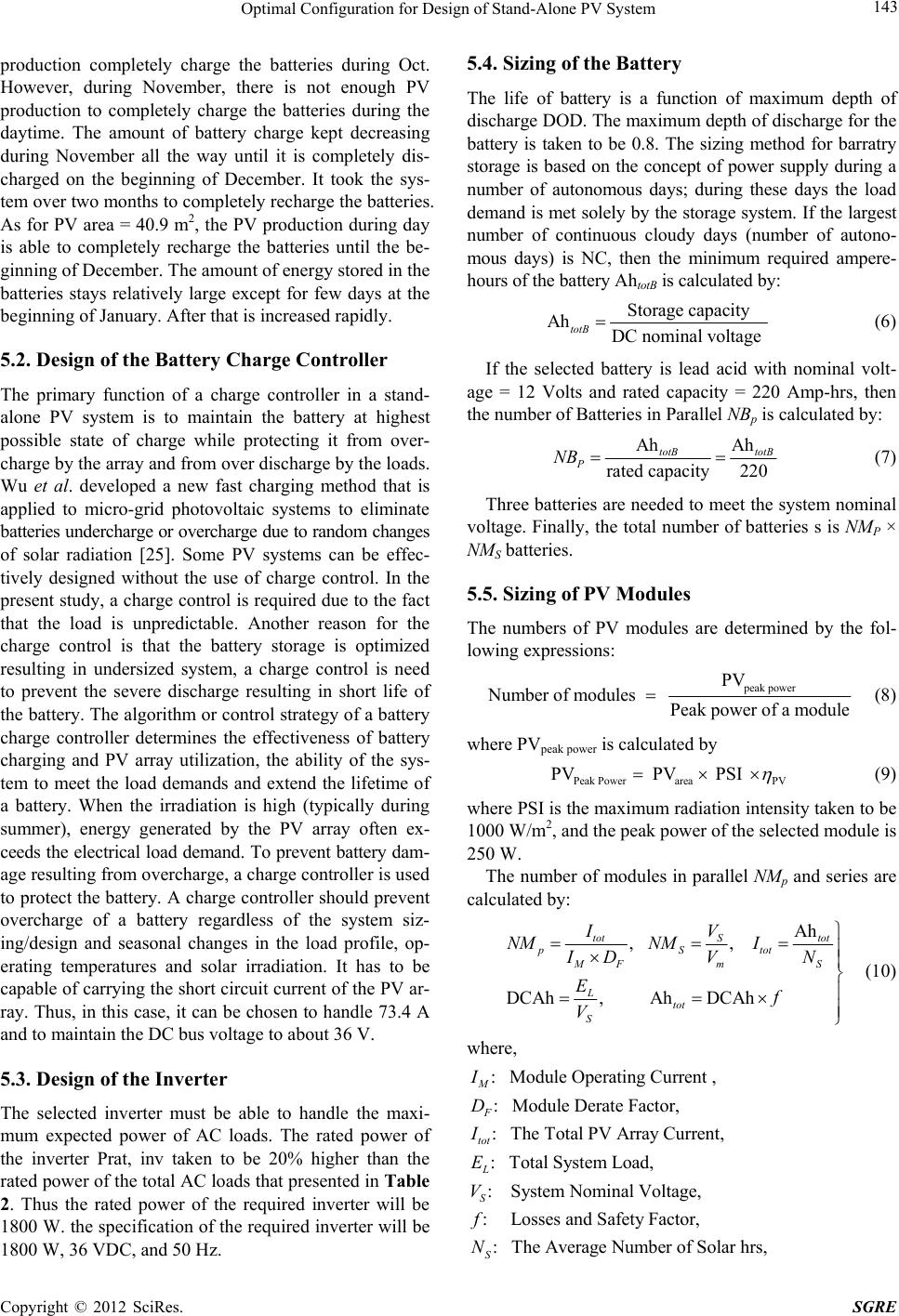

Optimal Configuration for Design of Stand-Alone PV System 143
production completely charge the batteries during Oct.
However, during November, there is not enough PV
production to completely charge the batteries during the
daytime. The amount of battery charge kept decreasing
during November all the way until it is completely dis-
charged on the beginning of December. It took the sys-
tem over two months to completely rech arge the batteries.
As for PV area = 40.9 m2, the PV production during day
is able to completely recharge the batteries until the be-
ginning of December. The amount of energy stored in the
batteries stays relatively large except for few days at the
beginning of January. After that is increased rapidly.
5.2. Design of the Battery Charge Controller
The primary function of a charge controller in a stand-
alone PV system is to maintain the battery at highest
possible state of charge while protecting it from over-
charge by the array and from over discharge by the loads.
Wu et al. developed a new fast charging method that is
applied to micro-grid photovoltaic systems to eliminate
batteries underch arge or overcharge due to random ch anges
of solar radiation [25]. Some PV systems can be effec-
tively designed without the use of charge control. In the
present study, a charge control is required due to the fact
that the load is unpredictable. Another reason for the
charge control is that the battery storage is optimized
resulting in undersized system, a charge control is need
to prevent the severe discharge resulting in short life of
the battery. The algorithm or control strategy of a battery
charge controller determines the effectiveness of battery
charging and PV array utilization, the ability of the sys-
tem to meet the load demands and extend the lifetime of
a battery. When the irradiation is high (typically during
summer), energy generated by the PV array often ex-
ceeds the electrical load demand. To prevent battery dam-
age resulting from overcharg e, a charge controller is used
to protect the battery. A charge controller should prevent
overcharge of a battery regardless of the system siz-
ing/design and seasonal changes in the load profile, op-
erating temperatures and solar irradiation. It has to be
capable of carrying the short circuit current of the PV ar-
ray. Thus, in this case, it can be chosen to hand le 73.4 A
and to maintain the DC bus voltage to about 36 V.
5.3. Design of the Inverter
The selected inverter must be able to handle the maxi-
mum expected power of AC loads. The rated power of
the inverter Prat, inv taken to be 20% higher than the
rated power of the total AC loads that presented in Table
2. Thus the rated power of the required inverter will be
1800 W. the specification of the required inverter will b e
1800 W, 36 VDC, and 50 Hz.
5.4. Sizing of the Battery
The life of battery is a function of maximum depth of
discharge DOD. The maximum depth of discharge for the
battery is taken to be 0.8. The sizing method for barratry
storage is based on the concept of power supply during a
number of autonomous days; during these days the load
demand is met solely by the sto rage system. If the largest
number of continuous cloudy days (number of autono-
mous days) is NC, then the minimum required ampere-
hours of the batt ery AhtotB is calculated by:
Storage capacity
Ah DC nominal voltage
totB  (6)
If the selected battery is lead acid with nominal volt-
age = 12 Volts and rated capacity = 220 Amp-hrs, then
the number of Batteries in Parallel NBp is calculated by:
Ah Ah
rated capacity220
totB totB
P
NB  (7)
Thre e batteries a re needed to meet the system nominal
voltage. Finally, the total number of batteries s is NMP ×
NMS batteries.
5.5. Sizing of PV Modules
The numbers of PV modules are determined by the fol-
lowing expressions:
peak power
PV
Number of modules Peak power of a module  (8)
where PVpeak power is calculated by
Peak PowerareaPV
PV PV PSI


 (9)
where PSI is the maximum radiation intensity take n to be
1000 W/m2, and the peak power of the selected module is
250 W.
The number of modules in parallel NMp and series are
calculated by:
Ah
, ,
DCAh, AhDCAh
totS tot
pStot
MFm S
L
tot
S
IV
NM NM I
IDV N
E f
V










(10)
where,
: Module Operating Current ,
: Module Derate Factor,
: The Total PV Array Current,
: Tot al System Load,
: System Nominal Voltage,
: Losses and Safety Factor,
: The Average Nu
M
F
tot
L
S
S
I
D
I
E
V
f
Nmber of Solar hrs,

Optimal Configuration for Design of Stand-Alone PV System
144
DCAh: The Total DC Amp-hours/Day,
: Number of Module in Series,
: Number of Module in Parallel.
S
P
NM
NM
NS is calculated from Table 1, to be 6 hours and the sys-
tem nominal voltage is taken to be 36 volt. The losses
and safety factor is assumed to be 1.2.
The total number of modules NMtot is
totP S
NMNM NM (11)
5.6. Sizing Optimization
As mentioned previously, the method presented here is
quit simple and quick, but the resulting sizing of the
combination of PV array and battery bank for a solar PV
system is not necessarily optimal. It is the objective of
this section to find a sizing combination that minimizes
the cost while maintaining desired values of reliability.
The reliability of power supply of system is expressed in
terms of the loss of load probability (LLP), defined as the
power failure time Tf divided by the estimated period of
time T, i.e. LLP = Tf/T. For the given LLP value of the
whole year, many configurations can meet this reliability
demand of power supply. In this study, a program for
calculating the LLP values and the total cost of different
configurations is developed. In the program, a PV area
and number of autonomous days are provided to the pro-
gram. The program calculates the daily PV output for the
whole year according to the following equation
PV
PVPV area
outinB Inv
G

   (12)
and compares it with the daily demand EL. A charge
controller is simulated that prevents the both overcharge
and the undercharge of batteries bank. The amount charge
stored in batteries is calculated daily. A power failure is
indicated if the amount of charge reaches the lower limits,
which is specified here to be 20% of the storage capacity
given by Equation (5). The program counts these times
and calculate LLP for the given combination. The pro-
gram calculates the total number of PV modules (paral-
lels and series) required according to Equations (10) and
(11).
The program has calculated the whole year’s LLP
values of different configurations with PV area changing
from 30 m2 to 50 m
2 and number of autonomous days
changing from 1 to 7. The trade-off curves between the
numbers of PV modules and number of batteries for
several LLPs are shown in Figure 5. Figure 5 shows
only parts of cal c ul at ion results.
The objective function of the optimization problem is
the life cycle cost (LCC) of stand-alone PV system. The
LCC of any system consists of the total costs of owning
and operating it over its lifetime, expressed in today’s
money. The costs of a stand-alone PV system include
acquisition costs, operating costs, maintenance costs, and
replacement costs. The LCC of the PV system includes
the sum of all the present worth’s (PWs) of the costs of
the PV modules, storage batteries, battery charger, and
inverter, the cost of the installation, and the maintenance
and operation cost (M&O) of the system. The details of
the used cost data for all items are shown in Table 3.
These data was obtained from the manufacturer of PV
system [26].
The lifetime N of all the items is considered to be 20
years, except that of the battery which is considered to be
5 years. Thus, an extra three groups have to be purchased,
after 5 years, 10 years, and 15 years. Assuming an infla-
tion rate i of 3% and an interest rate d of 10%.
The program calculates the LLC for any com binations
according to the following equations:
PV array cost CPV is given by:


PVPeak Power
242 $WPVC . 
(13)
where PVpeak power is calculated by Equation (9)
Initial cost of batteries is given by:


1 $AhAh
B
tot
C (14)
where Ahtot is the required ampere-hour of the batteries
calculated from Equation (6)


$0.5W
I
nvrat, inv
C P (15)
The charger cost is given by:


$0.5 W
C
CSC I

 (16)
15
17
19
21
23
25
27
29
31
258 111417
No. of Batteries
No. of PV modul e s
LLP = 0
LLP = 0. 011
LLP = 0. 022
LLP = 0. 03
LLP = 0. 033
LLP = 0. 049
Figure 5. Trade off curves between the numbers of batteries
and PV modules for the different LLP values.
Table 3. The used cost of all items.
M&O/
Year
Installation
Charge
controller
InverterBatteryPV Item
2% of
PV cost
10% of
PV cost
$3.2/A 0.5 $/W1$/Ah2.42 $/WCost

Optimal Configuration for Design of Stand-Alone PV System
145
The LCC of the system is calculated by summing all
the above cost, I’e
The installation cost is taken to be 10% of the PV co st.
As for the current value of the maintenance cost CMPW is
calculated by [25] : PV1PW 2PW
3PW MPW
LCC
BB B
BIns c inv
CCC C
CCCCC
 

(19)
  

 
MPW
11 1
1
Myr 1111
N
id
i
Cdi
 





 d
(17) Table 4 list sample of the calculation results output
from the program developed. For a given value of LLP
there is an optimum configuration that has the lowest
cost. For example, for LLP = 0.0027, the cost of the
combination that meet this requirement ranges from
$22,267 to 26,177. However, the optimum combination
is number of batteries = 10 and PV modules = 20. An-
other example for LLP = 0.033, the cost of the system
The maintenance cost per year (M/yr) is assumed 2%
of the PV cost.
The present value of the nth extra group of batteries
CBnPW purchased after N years is calculated by:
  
PW 11

N
Bn B
CCid (18)
Table 4. Sample of the calculation results.
PV area
(m2) No of autono- mous days Number of Batteries Number of PV modules LLP LLC ($)PV area (m2) No of autono- mous days Number of Batteries Number of PV modules LLPLLC ($)
35 4.5 11 20 0.00002323948.5 1 3 28 0.01124011
33.5 5 12 19 0.00002332050 1 3 29 0.01124679
45 3.5 9 26 0.00002619734 2 5 20 0.01419048
40 6 14 23 0.00002771434.5 2 5 20 0.01419270
50 6.5 15 29 0.00003292035.5 2 5 20 0.01419716
49.5 7 17 28 0.00003344631 5 12 18 0.01422206
50 7 17 29 0.00003366930.5 6 14 18 0.01423481
34.5 4 10 20 0.00272226730 7 17 17 0.01424757
35 4 10 20 0.00272249033.5 2 5 19 0.01918825
37 3.5 9 21 0.00272263232 2.5 6 18 0.01918905
37.5 3.5 9 22 0.00272285537.5 1.5 4 22 0.01919858
36 4 10 21 0.00272293538 1.5 4 22 0.01920081
33 5 12 19 0.00272309731 4 10 18 0.01920707
49.5 2 5 28 0.00272595531.5 2.5 6 18 0.02218683
50 2 5 29 0.00272617735 1.5 4 20 0.02218744
34 3.5 9 20 0.00552129537.5 1 3 22 0.02219109
34.5 3.5 9 20 0.00552151838 1 3 22 0.02219332
35 3.5 9 20 0.00552174131 3.5 9 18 0.02219958
37.5 3 7 22 0.00552210630.5 5.5 13 18 0.02222732
36 3.5 9 21 0.00552218634 1.5 4 20 0.02518298
39.5 2.5 6 23 0.00552224830.5 5 12 18 0.02521983
38 3 7 22 0.00552232830 5.5 13 17 0.02522509
33.5 4.5 11 19 0.00552257030 6 14 17 0.02523258
43 2 5 25 0.00552305835 1 3 20 0.02717995
49.5 1.5 4 28 0.00552520533.5 1.5 4 19 0.02718076
50 1.5 4 29 0.00552542830.5 4 10 18 0.02720484
34 3 7 20 0.00822054630.5 4.5 11 18 0.02721234
36 2.5 6 21 0.00822068830 5 12 17 0.02721760
34.5 3 7 20 0.00822076934.5 1 3 20 0.03017772
36.5 2.5 6 21 0.00822091133 1.5 4 19 0.03017853
35 3 7 20 0.00822099132 2 5 18 0.03018156
37 2.5 6 21 0.00822113430 4.5 11 17 0.03021011
39.5 2 5 23 0.00822149833 1 3 19 0.03317104
38 2.5 6 22 0.00822157931.5 1.5 4 18 0.03317184
38.5 2.5 6 22 0.00822180234 1 3 20 0.03317549
32 5 12 18 0.00822265131.5 2 5 18 0.03317934
44 1.5 4 25 0.00822275530 4 10 17 0.03320262
44.5 1.5 4 25 0.00822297731 1 3 18 0.04916212
34 2.5 6 20 0.01101979730.5 1.5 4 18 0.04916739
34.5 2.5 6 20 0.01102002030 2 5 17 0.04917265
35 2.5 6 20 0.01102024230 2.5 6 17 0.04918014

Optimal Configuration for Design of Stand-Alone PV System
146
ranges from $17,104 to $20,262. The op timum combina-
tion corresponds to number of b atteries = 3 and PV mod-
ules = 19. For LLP = 0, the stand-alone system works
without any power failure. The optimal cost for such sys-
tem is $23,239, which is comb ined of 11 batteries and 20
PV modules. However, for LLP = 0.049, which means
there are 18 nights without power in the whole year. The
optimal cost for such system is $16,212. Knowing this
difference can help the designer decided to install an-
other auxiliary hybrid system or not.
It is sometimes useful to calculate th e LCC of a system
on an annual basis. The annualized LCC (ALCC) of the
PV system in terms of the present day dollars can be
calculated by:
11
ALCCLCC 11
11
N
i
dd



 
 


  


 




i




(20)
Unit electrical cost of 1 kWh is ALCC
365
L
E.
Table 5 summarizes the optimal configurations and
the corresponding unit cost of electricity. The calculated
current unit cost of PV systems depends on the LLP val-
ues. There values range b etween 0.419 S/kWh and 0.293
$/kWh. Although this price is very high compared to the
current unit cost of electricity in Jordan (0 .114 $/kWh), it
is predicted that this price will drop significantly in the
future due to decrease in the initial cost of the PV mod-
ules. At the same time, if the future unit cost of electric-
ity in Jordan increases due to the rapid increase in the
conventional fuel prices, therefore PV energy generation
will be promising in the future house electrification due
to its expected future lo wer unit electricity cost, efficiency
increase, and clean energy generation compared to the
convention al utility grid.
6. Conclusion
An electrification study for a single residential house in a
remote isolated site of Jordan is carried out using a
Table 5. Summary of the optimal configurations size and
cost for given LLPs.
PV
area (m2)
No of
Autonomous
Days
Number
of
Batteries
Number
of PV
Modules LLP LLC ($)Cost of
1 kWh
35 4.5 11 20 0.0000 232390.419
34.5 4 10 20 0.0027 222670.402
34 3.5 9 20 0.0055 212950.384
34 3 7 20 0.0082 205460.371
34 2 5 20 0.014 190480.344
34.5 1 3 20 0.030 177720.321
33 1 3 19 0.033 171040.309
31 1 3 18 0.049 162120.293
stand-alone PV system. The complete design steps and
the life cycle cost analysis of the PV system is presented.
A method based on calculating the yearly loss of load
probability LLP has been presented for a PV sizing. A
computer program that simulates the stand-alone PV
system daily behavior is developed. According to local
hourly measured meteorological data, load demand, the
characteristic and price of the components and reliability
requirement on power sup ply, the optimum configu ration
which meets the load demand with the minimum cost can
be uniquely determined by the program. The unit electri-
cal cost for electrifying a remote isolated house using PV
systems is calculated. The results of study indicates that
using the optimal configuration for electrifying remote
areas in Jordan is beneficial and suitable for long-term
investments, especially if the in itial prices of the PV sys-
tems are decreased and their efficiencies are increased.
Therefore, in remote sites that are too far from the Jorda-
nian power grid, it is encouraged to in stall PV systems to
generate electricity.
REFERENCES
[1] A. Guglielmo, S. Stefano Redi, A. Tatnall and T. Markvart,
“Harnessing High-Altitude Solar Power,” IEEE Transac-
tions Energy Conversion, Vol. 24, No. 2, 2009, pp. 442-451.
doi:10.1109/TEC.2009.2016026
[2] G. C. Bakos and M. Soursos, “Techno-Economic Assess-
ment of a Stand-Alone PV/Hybrid Installation for Low-
Cost Electrification of a Tourist Resort in Greece,” Ap-
plied Energy, Vol. 73, No. 2, 2002, pp. 183-193.
doi:10.1016/S0306-2619(02)00062-4
[3] W. M. Rohouma, I. M. Molokhia and A. H. Esuri, “Com-
parative Study of Different PV Modules Configuration
Reliability,” Desalination, Vol. 209, No. 1-3, 2007, pp.
122-128. doi:10.1016/j.desal.2007.04.020
[4] D. Lowe and C. R. Lloyd, “Renewable Energy Systems
for Remote Areas in Australia,” Renew Energy, Vol. 22,
No. 1-3, 2001, pp. 369-378.
doi:10.1016/S0960-1481(00)00043-4
[5] Jordan Meteorological Department, “Jordan Annual Cli-
mate JMD,” Amman, Jordan, 1998.
[6] S. Silvestre, “Review of System Design and Sizing Tools.
Practical Handbook of Photovoltaics: Fundamentals and
Applications,” Elsevier, Oxford, 2003, 543 p.
[7] M. Egido and E. Lorenzo, “The Sizing of a Stand-Alone
PV Systems: A Review and A Proposed New Method,”
Solar Energy Materials and Solar Cells, Vol. 26, No. 1-2,
1992, pp. 51-69. doi:10.1016/0927-0248(92)90125-9
[8] R. Posadillo and R. Luque, “Approaches for Developing a
Sizing Method for Stand-Alone PV Systems with Vari-
able Demand,” Renewable Energy, Vol. 33, No. 5, 2008,
pp. 1037-1048. doi:10.1016/j.renene.2007.06.004
[9] E. Ofry and A. Braunstein, “The Loss of Power Supply
Probability as a Technique for Stand-Alone Solar Elec-
trical (Photovoltaic) Systems,” IEEE Transactions on Power

Optimal Configuration for Design of Stand-Alone PV System 147
Apparatus and Systems, Vol. 102, No. 5, 1983, pp. 1171-
1175. doi:10.1109/TPAS.1983.318057
[10] L. L. Bucciarelli Jr., “Estimating Loss-of-Power Probabil-
ities of Stand-Alone Photovoltaic Solar Energy Systems,”
Solar Energy, Vol. 32, No. 2, 1984, pp. 205-209.
doi:10.1016/S0038-092X(84)80037-7
[11] L. Barra, S. Catalanotti, F. Fontana and F. Lavorante,” An
Analytical Method to Determine the Optimal Size of a
Photovoltaic Plant,” Solar Energy, Vol. 33, No. 6, 1984,
pp. 509-514. doi:10.1016/0038-092X(84)90005-7
[12] B. Bartoli, V. Cuomo, F. Fontana, C. Serio and V. Silves-
trini, “The Design of Photovoltaic Plants: An Optimiza-
tion Procedure,” Applied Energy, Vol. 18, No. 1, 1984, pp.
37-47. doi:10.1016/0306-2619(84)90044-8
[13] M. Cardona and L. L. López, “A Simple Model for Sizing
Stand-Alone Photovoltaic Systems,” Solar Energy Mate-
rials and Solar Cells, Vol. 55, No. 3, 1998, pp. 199-214.
doi:10.1016/S0927-0248(98)00093-2
[14] Chapman, “Sizing Handbook for Stand-Alone Photovol-
taic/Storage Systems,” Sandia National Laboratories, 1987.
[15] M. Sidrach-de-Cardona and L. L. Mora López, “A Gen-
eral Multivariate Qualitative Model for Sizing Stand-
Alone Photovoltaic Systems,” Solar Energy Materials and
Solar Cells, Vol. 59, No. 3, 1999, pp. 185-197.
doi:10.1016/S0927-0248(99)00020-3
[16] I. Abouzahr and R. Ramkumar, “Loss of Power Supply
Probability of Stand-Alone Photovoltaic Systems: A Closed
Form Solution Approach,” IEEE Transactions on Energy
Conversion, Vol. 6, No. 1, 1991, pp. 1-11.
doi:10.1109/60.73783
[17] S. A. Klein and W. A. Beckman, “Loss-of-Load Prob-
abilities for Stand-Alone Photovoltaic Systems,” Solar
Energy, Vol. 39, No. 6, 1987, pp. 499-512.
doi:10.1016/0038-092X(87)90057-0
[18] F. Hernández and M. Hernández-Campos, “The Devel-
opment of the Renewable Energy Technologies in Spain,”
Smart Grid and Renewable Energy, Vol. 2, No. 2, 2011,
pp. 110-115. doi:10.4236/sgre.2011.22013
[19] R. Chenni, E. Matagne and M. Khennane, “Study of Solar
Radiation in View of Photovoltaic Systems Optimiza-
tion,” Smart Grid and Renewable Energy, Vol. 2, No. 4,
2011, pp. 367-374. doi:10.4236/sgre.2011.24042
[20] J. E. Hay, “Calculation of Monthly Mean Solar Radiation
for Horizontal and Inclined Surface,” Solar Energy, Vol.
23, No. 4, 1979, pp. 301-308.
doi:10.1016/0038-092X(79)90123-3
[21] T. M. I. Alamsyah, K. Sopian and A. Sha hrir, “In Techno-
economics Analysis of a Photovoltaic System to Provide
Electricity for a Household in Malaysia,” Proceedings of
the International Symposium on Renewable Energy: En-
vironment Protection & Energy Solution for Sustainable
Development, Kuala Lumpur, 2003, pp. 387-396.
[22] M. Kolhe, “Techno-Economic Optimum Sizing of a Stand-
Alone Solar Photovoltaic System,” IEEE Transactions on
Energy Conversion, Vol. 24, No. 2, 2009, pp. 511-519.
doi:10.1109/TEC.2008.2001455
[23] S. R. Wenham, M. A. Green and M. E. Watt, “Applied
Photovoltaics,” Center for Photovoltaic Devices and Sys-
tems, Australia, 1994.
[24] Philadelphia. http://solar.com/default.aspx
[25] R. Messenger and J. Ventre, “Photovoltaic Systems En-
gineering, CRC,” Press LLC, Boca Raton, 2000.
[26] T. Wu, Q. Xiao, L. Wu, J. Zhang and M. Wang, “Study and
Implementation on Batteries Charging Method of Micro-
Grid Photovoltaic Systems,” Smart Grid and Renewable
Energy, Vol. 2, No. 4, 2011, pp.324-329.