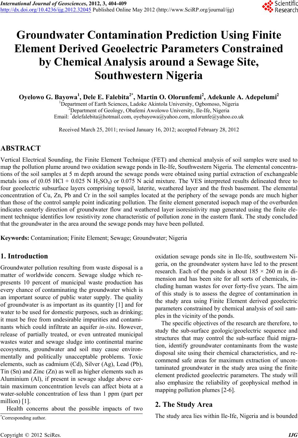
International Journal of Geosciences, 2012, 3, 404-409
http://dx.doi.org/10.4236/ijg.2012.32045 Published Online May 2012 (http://www.SciRP.org/journal/ijg)
Groundwater Contamination Prediction Using Finite
Element Derived Geoelectric Parameters Constrained
by Chemical Analysis around a Sewage Site,
Southwestern Nigeria
Oyelowo G. Bayowa1, Dele E. Falebita2*, Martin O. Olorunfemi2, Adekunle A. Adepelumi2
1Department of Earth Sciences, Ladoke Akintola University, Ogbomoso, Nigeria
2Department of Geology, Obafemi Awolowo University, Ile-Ife, Nigeria
Received March 25, 2011; revised January 16, 2012; accepted February 28, 2012
ABSTRACT
Vertical Electrical Sounding, the Finite Element Technique (FET) and chemical analysis of soil samples were used to
map the pollution plume around two oxidation sewage ponds in Ile-Ife, Southwestern Nigeria. The elemental concentra-
tions of the soil samples at 5 m depth around the sewage ponds were obtained using partial extraction of exchangeable
metals ions of (0.05 HCl + 0.025 N H2SO4) or 0.075 N acid mixture. The VES interpreted results delineated three to
four geoelectric subsurface layers comprising topsoil, laterite, weathered layer and the fresh basement. The elemental
concentration of Cu, Zn, Pb and Cr in the soil samples located at the periphery of the sewage ponds are much higher
than those of the control sample point indicating pollution. The finite element generated isopach map of the overburden
indicates easterly direction of groundwater flow and weathered layer isoresistivity map generated using the finite ele-
ment technique identifies low resistivity zone characteristic of pollution zone in the eastern flank. The study concluded
that the groundwater in the area around the sewage ponds may have been polluted.
Keywords: Contamination; Finite Element; Sewage; Groundwater; Nigeria
1. Introduction
Groundwater pollution resulting from waste disposal is a
matter of worldwide concern. Sewage sludge which re-
presents 10 percent of municipal waste production has
every chance of contaminating the groundwater which is
an important source of public water supply. The quality
of groundwater is as important as its quantity [1] and for
water to be used for domestic purposes, such as drinking;
it must be free from undesirable impurities and contami-
nants which could infiltrate an aquifer in-situ. However,
release of partially treated, or even untreated municipal
wastes water and sewage sludge into continental marine
ecosystems, groundwater and soil may cause environ-
mentally and politically unacceptable problems. Toxic
elements, such as cadmium (Cd), Silver (Ag), Lead (Pb),
Tin (Sn) and Zinc (Zn) as well as higher elements such as
Aluminium (Al), if present in sewage sludge above cer-
tain maximum concentration levels can affect biota at a
water-soluble concentration of less than 1 ppm (part per
million) [1].
Health concerns about the possible impacts of two
oxidation sewage ponds site in Ile-Ife, southwestern Ni-
geria, on the groundwater system have led to the present
research. Each of the ponds is about 185 × 260 m in di-
mension and has been site for all sorts of chemicals, in-
cluding human wastes for over forty-five years. The aim
of this study is to assess the degree of contamination in
the study area using Finite Element derived geoelectric
parameters constrained by chemical analysis of soil sam-
ples in the vicinity of the ponds.
The specific objectives of the research are therefore, to
study the sub-surface geologic/geoelectric sequence and
structures that may control the sub-surface fluid migra-
tion, identify groundwater contaminants from the waste
disposal site using their chemical characteristics, and re-
commend safe areas for maximum extraction of uncon-
taminated groundwater in the study area using the finite
element predicted geoelectric parameters. The study will
also emphasize the reliability of geophysical method in
mapping pollution plumes [2-6].
2. The Study Area
The study area lies within Ile-Ife, Nigeria and is bounded
*Corresponding author.
C
opyright © 2012 SciRes. IJG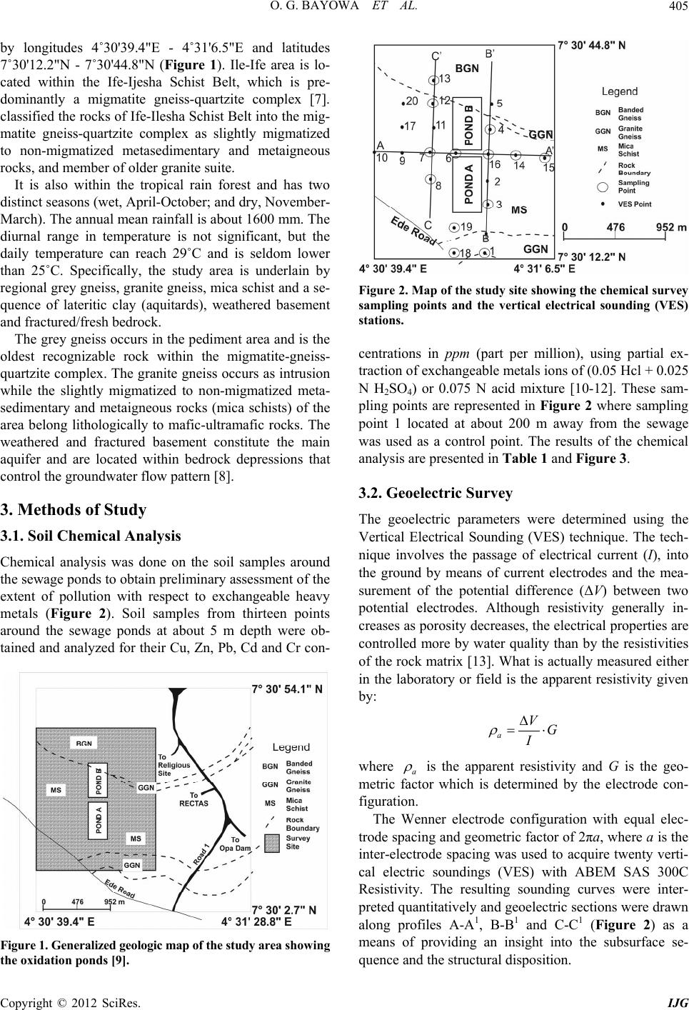

O. G. BAYOWA ET AL. 405
by longitudes 4˚30'39.4"E - 4˚31'6.5"E and latitudes
7˚30'12.2"N - 7˚30'44.8"N (Figure 1). Ile-Ife area is lo-
cated within the Ife-Ijesha Schist Belt, which is pre-
dominantly a migmatite gneiss-quartzite complex [7].
classified the rocks of Ife-Ilesha Schist Belt into the mig-
matite gneiss-quartzite complex as slightly migmatized
to non-migmatized metasedimentary and metaigneous
rocks, and member of older granite suite.
It is also within the tropical rain forest and has two
distinct seasons (wet, April-October; and dry, November-
March). The annual mean rainfall is about 1600 mm. The
diurnal range in temperature is not significant, but the
daily temperature can reach 29˚C and is seldom lower
than 25˚C. Specifically, the study area is underlain by
regional grey gneiss, granite gneiss, mica schist and a se-
quence of lateritic clay (aquitards), weathered basement
and fractured/fresh bedrock.
The grey gneiss occurs in the pediment area and is the
oldest recognizable rock within the migmatite-gneiss-
quartzite complex. The granite gneiss occurs as intrusion
while the slightly migmatized to non-migmatized meta-
sedimentary and metaigneous rocks (mica schists) of the
area belong lithologically to mafic-ultramafic rocks. The
weathered and fractured basement constitute the main
aquifer and are located within bedrock depressions that
control the groundwater flow pattern [8].
3. Methods of Study
3.1. Soil Chemical Analysis
Chemical analysis was done on the soil samples around
the sewage ponds to obtain preliminary assessment of the
extent of pollution with respect to exchangeable heavy
metals (Figure 2). Soil samples from thirteen points
around the sewage ponds at about 5 m depth were ob-
tained and analyzed for their Cu, Zn, Pb, Cd and Cr con-
Figure 1. Generalized geologic map of the study area showing
the oxidation ponds [9].
Figure 2. Map of the study site showing the chemical survey
sampling points and the vertical electrical sounding (VES)
stations.
centrations in ppm (part per million), using partial ex-
traction of exchangeable metals ions of (0.05 Hcl + 0.025
N H2SO4) or 0.075 N acid mixture [10-12]. These sam-
pling points are represented in Figure 2 where sampling
point 1 located at about 200 m away from the sewage
was used as a control point. The results of the chemical
analysis are presented in Table 1 and Figure 3.
3.2. Geoelectric Survey
The geoelectric parameters were determined using the
Vertical Electrical Sounding (VES) technique. The tech-
nique involves the passage of electrical current (I), into
the ground by means of current electrodes and the mea-
surement of the potential difference (ΔV) between two
potential electrodes. Although resistivity generally in-
creases as porosity decreases, the electrical properties are
controlled more by water quality than by the resistivities
of the rock matrix [13]. What is actually measured either
in the laboratory or field is the apparent resistivity given
by:
aVG
I




where a

is the apparent resistivity and G is the geo-
metric factor which is determined by the electrode con-
figuration.
The Wenner electrode configuration with equal elec-
trode spacing and geometric factor of 2πa, where a is the
inter-electrode spacing was used to acquire twenty verti-
cal electric soundings (VES) with ABEM SAS 300C
Resistivity. The resulting sounding curves were inter-
preted quantitatively and geoelectric sections were drawn
along profiles A-A1, B-B1 and C-C1 (Figure 2) as a
means of providing an insight into the subsurface se-
quence and the structural disposition.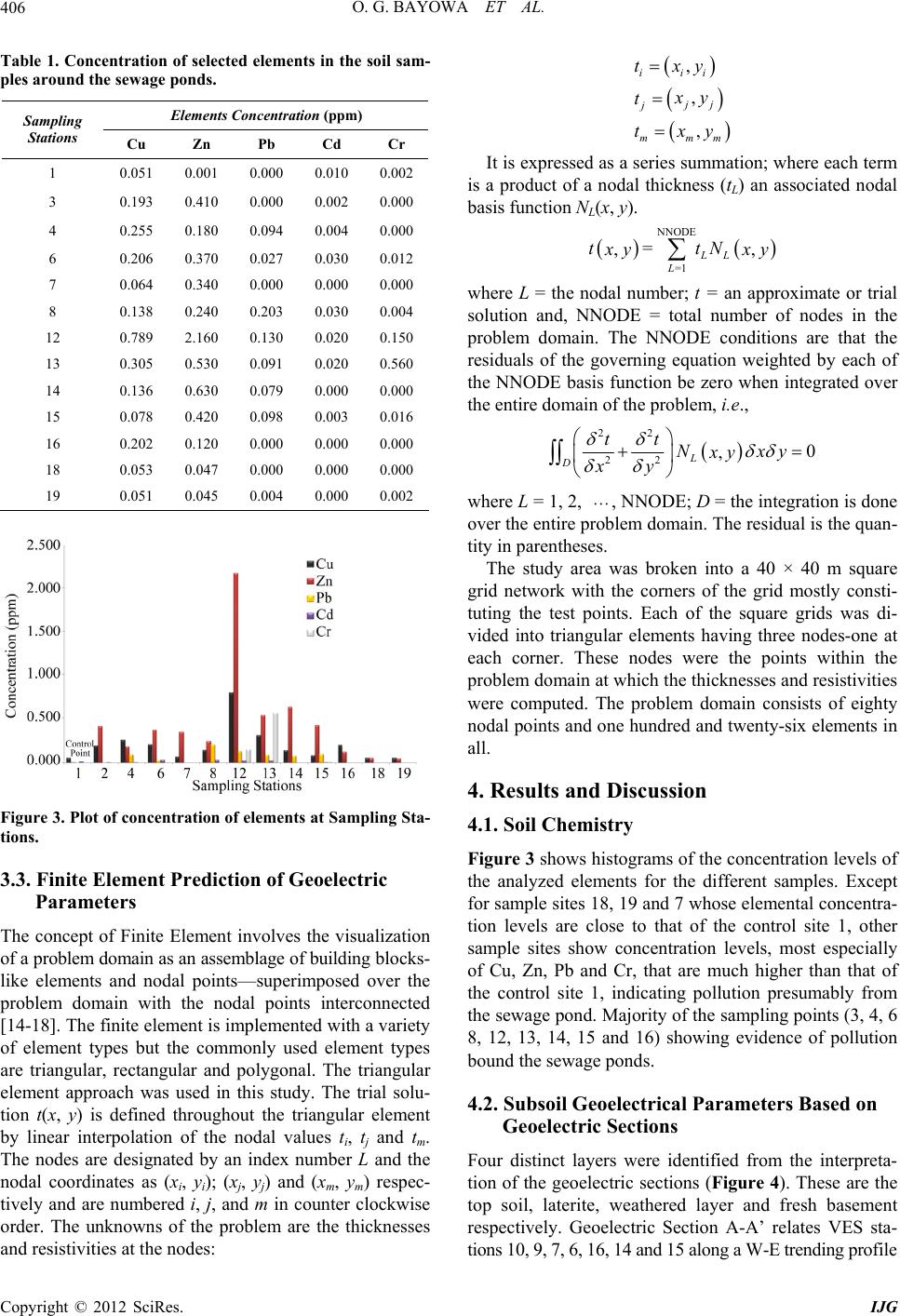

O. G. BAYOWA ET AL. 406




,
,
,
iii
jj j
mmm
txy
Table 1. Concentration of selected elements in the soil sam-
ples around the sew age ponds.
x
y
t
txy



 
NNODE
1
, ,
LL
L=
t = tN
Elements Concentration (ppm)
Sampling
Stations Cu Zn Pb Cd Cr
1 0.051 0.001 0.000 0.010 0.002
3 0.193 0.410 0.000 0.002 0.000
4 0.255 0.180 0.094 0.004 0.000
6 0.206 0.370 0.027 0.030 0.012
7 0.064 0.340 0.000 0.000 0.000
8 0.138 0.240 0.203 0.030 0.004
12 0.789 2.160 0.130 0.020 0.150
13 0.305 0.530 0.091 0.020 0.560
14 0.136 0.630 0.079 0.000 0.000
15 0.078 0.420 0.098 0.003 0.016
16 0.202 0.120 0.000 0.000 0.000
18 0.053 0.047 0.000 0.000 0.000
19 0.051 0.045 0.004 0.000 0.002
Figure 3. Plot of concentration of elements at Sampling Sta-
tions.
3.3. Finite Element Prediction of Geoelectric
Parameters
The concept of Finite Element involves the visualization
of a problem domain as an assemblage of building blocks-
like elements and nodal points—superimposed over the
problem domain with the nodal points interconnected
[14-18]. The finite element is implemented with a variety
of element types but the commonly used element types
are triangular, rectangular and polygonal. The triangular
element approach was used in this study. The trial solu-
tion t(x, y) is defined throughout the triangular element
by linear interpolation of the nodal values ti, tj and tm.
The nodes are designated by an index number L and the
nodal coordinates as (xi, yi); (xj, yj) and (xm, ym) respec-
tively and are numbered i, j, and m in counter clockwise
order. The unknowns of the problem are the thicknesses
and resistivities at the nodes:
It is expressed as a series summation; where each term
is a product of a nodal thickness (tL) an associated nodal
basis function NL(x, y).
yxy

x
where L = the nodal number; t = an approximate or trial
solution and, NNODE = total number of nodes in the
problem domain. The NNODE conditions are that the
residuals of the governing equation weighted by each of
the NNODE basis function be zero when integrated over
the entire domain of the problem, i.e.,

22
22 0
,
L
D
tt
Nxy xy
xy
 








where L = 1, 2, , NNODE; D = the integration is done
over the entire problem domain. The residual is the quan-
tity in parentheses.
The study area was broken into a 40 × 40 m square
grid network with the corners of the grid mostly consti-
tuting the test points. Each of the square grids was di-
vided into triangular elements having three nodes-one at
each corner. These nodes were the points within the
problem domain at which the thicknesses and resistivities
were computed. The problem domain consists of eighty
nodal points and one hundred and twenty-six elements in
all.
4. Results and Discussion
4.1. Soil Chemistry
Figure 3 shows histograms of the concentration levels of
the analyzed elements for the different samples. Except
for sample sites 18, 19 and 7 whose elemental concentra-
tion levels are close to that of the control site 1, other
sample sites show concentration levels, most especially
of Cu, Zn, Pb and Cr, that are much higher than that of
the control site 1, indicating pollution presumably from
the sewage pond. Majority of the sampling points (3, 4, 6
8, 12, 13, 14, 15 and 16) showing evidence of pollution
bound the sewage ponds.
4.2. Subsoil Geoelectrical Parameters Based on
Geoelectric Sections
Four distinct layers were identified from the interpreta-
tion of the geoelectric sections (Figure 4). These are the
top soil, laterite, weathered layer and fresh basement
respectively. Geoelectric Section A-A’ relates VES sta-
tions 10, 9, 7, 6, 16, 14 and 15 along a W-E trending profile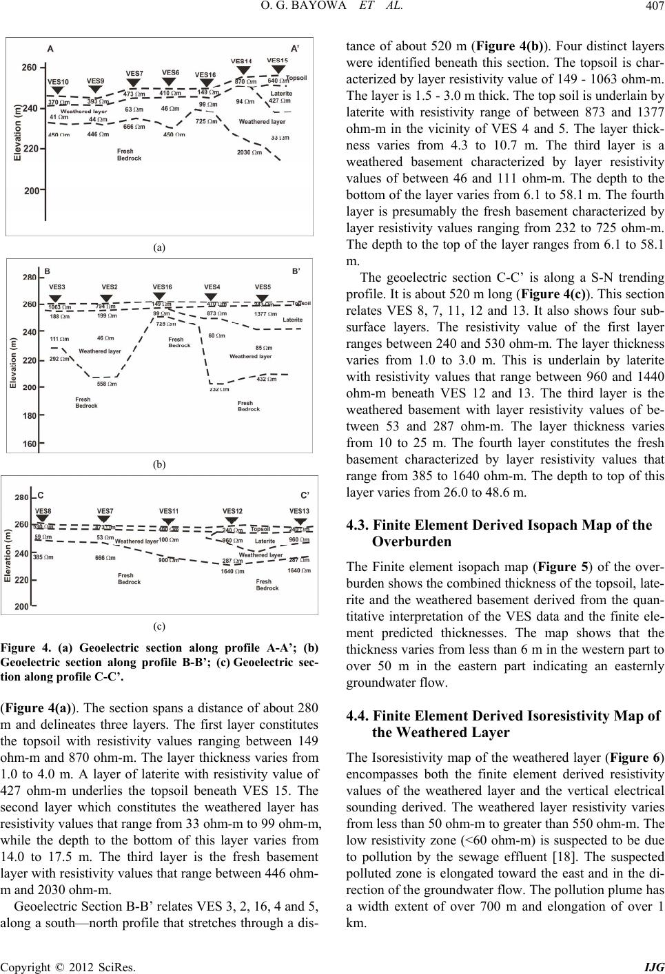

O. G. BAYOWA ET AL. 407
(a)
(b)
(c)
Figure 4. (a) Geoelectric section along profile A-A’; (b)
Geoelectric section along profile B-B’; (c) Geoelectric sec-
tion along profile C-C’.
(Figure 4(a)). The section spans a distance of about 280
m and delineates three layers. The first layer constitutes
the topsoil with resistivity values ranging between 149
ohm-m and 870 ohm-m. The layer thickness varies from
1.0 to 4.0 m. A layer of laterite with resistivity value of
427 ohm-m underlies the topsoil beneath VES 15. The
second layer which constitutes the weathered layer has
resistivity values that range from 33 ohm-m to 99 ohm-m,
while the depth to the bottom of this layer varies from
14.0 to 17.5 m. The third layer is the fresh basement
layer with resistivity values that range between 446 ohm-
m and 2030 ohm-m.
Geoelectric Section B-B’ relates VES 3, 2, 16, 4 and 5,
along a south—north profile that stretches through a dis-
tance of about 520 m (Figure 4(b)). Four distinct layers
were identified beneath this section. The topsoil is char-
acterized by layer resistivity value of 149 - 1063 ohm-m.
The layer is 1.5 - 3.0 m thick. The top soil is underlain by
laterite with resistivity range of between 873 and 1377
ohm-m in the vicinity of VES 4 and 5. The layer thick-
ness varies from 4.3 to 10.7 m. The third layer is a
weathered basement characterized by layer resistivity
values of between 46 and 111 ohm-m. The depth to the
bottom of the layer varies from 6.1 to 58.1 m. The fourth
layer is presumably the fresh basement characterized by
layer resistivity values ranging from 232 to 725 ohm-m.
The depth to the top of the layer ranges from 6.1 to 58.1
m.
The geoelectric section C-C’ is along a S-N trending
profile. It is about 520 m long (Figure 4(c)). This section
relates VES 8, 7, 11, 12 and 13. It also shows four sub-
surface layers. The resistivity value of the first layer
ranges between 240 and 530 ohm-m. The layer thickness
varies from 1.0 to 3.0 m. This is underlain by laterite
with resistivity values that range between 960 and 1440
ohm-m beneath VES 12 and 13. The third layer is the
weathered basement with layer resistivity values of be-
tween 53 and 287 ohm-m. The layer thickness varies
from 10 to 25 m. The fourth layer constitutes the fresh
basement characterized by layer resistivity values that
range from 385 to 1640 ohm-m. The depth to top of this
layer varies from 26.0 to 48.6 m.
4.3. Finite Element Derived Isopach Map of the
Overburden
The Finite element isopach map (Figure 5) of the over-
burden shows the combined thickness of the topsoil, late-
rite and the weathered basement derived from the quan-
titative interpretation of the VES data and the finite ele-
ment predicted thicknesses. The map shows that the
thickness varies from less than 6 m in the western part to
over 50 m in the eastern part indicating an easternly
groundwater flow.
4.4. Finite Element Derived Isoresistivity Map of
the Weathered Layer
The Isoresistivity map of the weathered layer (Figure 6)
encompasses both the finite element derived resistivity
values of the weathered layer and the vertical electrical
sounding derived. The weathered layer resistivity varies
from less than 50 ohm-m to greater than 550 ohm-m. The
low resistivity zone (<60 ohm-m) is suspected to be due
to pollution by the sewage effluent [18]. The suspected
polluted zone is elongated toward the east and in the di-
rection of the groundwater flow. The pollution plume has
a width extent of over 700 m and elongation of over 1
km.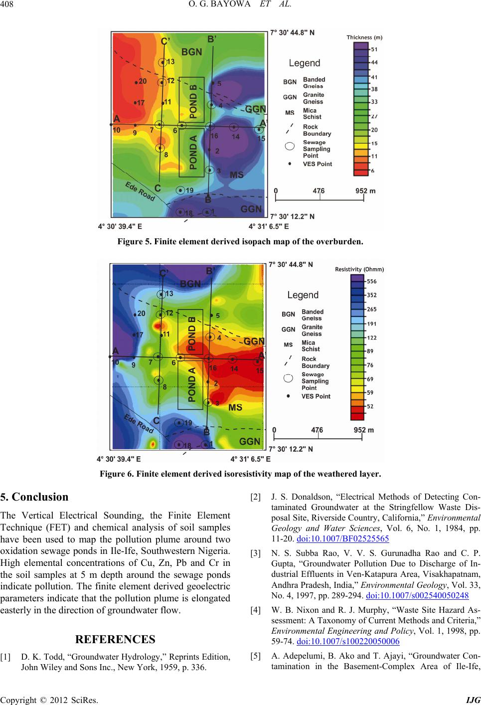

O. G. BAYOWA ET AL. 408
Figure 5. Finite elem e nt der ived isopach map of the overbur de n.
Figure 6. Finite element derived isoresistivity map of the weathered layer.
5. Conclusion [2] J. S. Donaldson, “Electrical Methods of Detecting Con-
taminated Groundwater at the Stringfellow Waste Dis-
posal Site, Riverside Country, California,” Environmental
Geology and Water Sciences, Vol. 6, No. 1, 1984, pp.
11-20. doi:10.1007/BF02525565
The Vertical Electrical Sounding, the Finite Element
Technique (FET) and chemical analysis of soil samples
have been used to map the pollution plume around two
oxidation sewage ponds in Ile-Ife, Southwestern Nigeria.
High elemental concentrations of Cu, Zn, Pb and Cr in
the soil samples at 5 m depth around the sewage ponds
indicate pollution. The finite element derived geoelectric
parameters indicate that the pollution plume is elongated
easterly in the direction of groundwater flow.
[3] N. S. Subba Rao, V. V. S. Gurunadha Rao and C. P.
Gupta, “Groundwater Pollution Due to Discharge of In-
dustrial Effluents in Ven-Katapura Area, Visakhapatnam,
Andhra Pradesh, India,” Environmental Geology, Vol. 33,
No. 4, 1997, pp. 289-294. doi:10.1007/s002540050248
[4] W. B. Nixon and R. J. Murphy, “Waste Site Hazard As-
sessment: A Taxonomy of Current Methods and Criteria,”
Environmental Engineering and Policy, Vol. 1, 1998, pp.
59-74. doi:10.1007/s100220050006
REFERENCES
[5] A. Adepelumi, B. Ako and T. Ajayi, “Groundwater Con-
tamination in the Basement-Complex Area of Ile-Ife,
[1] D. K. Todd, “Groundwater Hydrology,” Reprints Edition,
John Wiley and Sons Inc., New York, 1959, p. 336.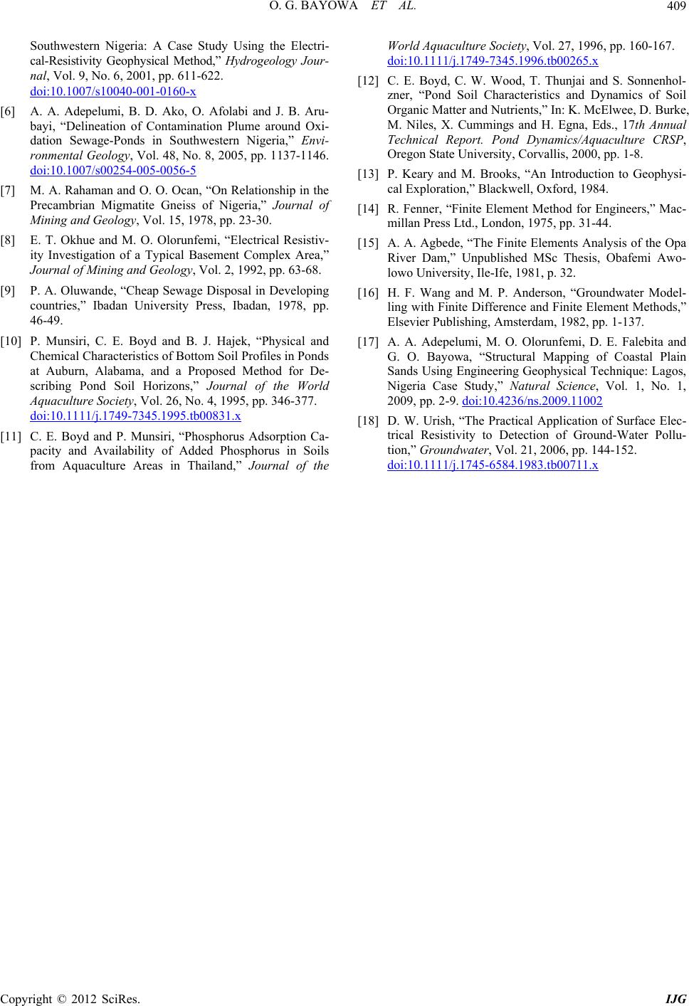

O. G. BAYOWA ET AL. 409
Southwestern Nigeria: A Case Study Using the Electri-
cal-Resistivity Geophysical Method,” Hydrogeology Jour-
nal, Vol. 9, No. 6, 2001, pp. 611-622.
doi:10.1007/s10040-001-0160-x
[6] A. A. Adepelumi, B. D. Ako, O. Afolabi and J. B. Aru-
bayi, “Delineation of Contamination Plume around Oxi-
dation Sewage-Ponds in Southwestern Nigeria,” Envi-
ronmental Geology, Vol. 48, No. 8, 2005, pp. 1137-1146.
doi:10.1007/s00254-005-0056-5
[7] M. A. Rahaman and O. O. Ocan, “On Relationship in the
Precambrian Migmatite Gneiss of Nigeria,” Journal of
Mining and Geology, Vol. 15, 1978, pp. 23-30.
[8] E. T. Okhue and M. O. Olorunfemi, “Electrical Resistiv-
ity Investigation of a Typical Basement Complex Area,”
Journal of Mining and Geology, Vol. 2, 1992, pp. 63-68.
[9] P. A. Oluwande, “Cheap Sewage Disposal in Developing
countries,” Ibadan University Press, Ibadan, 1978, pp.
46-49.
[10] P. Munsiri, C. E. Boyd and B. J. Hajek, “Physical and
Chemical Characteristics of Bottom Soil Profiles in Ponds
at Auburn, Alabama, and a Proposed Method for De-
scribing Pond Soil Horizons,” Journal of the World
Aquaculture Society, Vol. 26, No. 4, 1995, pp. 346-377.
doi:10.1111/j.1749-7345.1995.tb00831.x
[11] C. E. Boyd and P. Munsiri, “Phosphorus Adsorption Ca-
pacity and Availability of Added Phosphorus in Soils
from Aquaculture Areas in Thailand,” Journal of the
World Aquaculture Society, Vol. 27, 1996, pp. 160-167.
doi:10.1111/j.1749-7345.1996.tb00265.x
[12] C. E. Boyd, C. W. Wood, T. Thunjai and S. Sonnenhol-
zner, “Pond Soil Characteristics and Dynamics of Soil
Organic Matter and Nutrients,” In: K. McElwee, D. Burke,
M. Niles, X. Cummings and H. Egna, Eds., 17th Annual
Technical Report. Pond Dynamics/Aquaculture CRSP,
Oregon State University, Corvallis, 2000, pp. 1-8.
[13] P. Keary and M. Brooks, “An Introduction to Geophysi-
cal Exploration,” Blackwell, Oxford, 1984.
[14] R. Fenner, “Finite Element Method for Engineers,” Mac-
millan Press Ltd., London, 1975, pp. 31-44.
[15] A. A. Agbede, “The Finite Elements Analysis of the Opa
River Dam,” Unpublished MSc Thesis, Obafemi Awo-
lowo University, Ile-Ife, 1981, p. 32.
[16] H. F. Wang and M. P. Anderson, “Groundwater Model-
ling with Finite Difference and Finite Element Methods,”
Elsevier Publishing, Amsterdam, 1982, pp. 1-137.
[17] A. A. Adepelumi, M. O. Olorunfemi, D. E. Falebita and
G. O. Bayowa, “Structural Mapping of Coastal Plain
Sands Using Engineering Geophysical Technique: Lagos,
Nigeria Case Study,” Natural Science, Vol. 1, No. 1,
2009, pp. 2-9. doi:10.4236/ns.2009.11002
[18] D. W. Urish, “The Practical Application of Surface Elec-
trical Resistivity to Detection of Ground-Water Pollu-
tion,” Groundwater, Vol. 21, 2006, pp. 144-152.
doi:10.1111/j.1745-6584.1983.tb00711.x