Modern Economy, 2012, 3, 284-294
http://dx.doi.org/10.4236/me.2012.33038 Published Online May 2012 (http://www.SciRP.org/journal/me)
VIX and VIX Futures Pricing Algorithms: Cultivating
Understanding
G. D’Anne Hancock
Finance University of Missouri-St. Louis, St. Louis, USA
Received April 2, 2012; revised April 19, 2012; accepted May 3, 2012
ABSTRACT
This article reviews the development of the S&P 500 volatility index and uses market information to develop algorithms
which aid in clarifying some of the salient points in the determination of an index value. Understanding the pertinent
points provides insigh t into the interpretation and limitations of the usefulness of the VIX and other VIX-type contracts.
Keywords: VIX Pricing; VIX Futures; VIX Options; Volatility Index
1. Introduction
This article reviews the development of the S&P 500
volatility index and the VIX futures contracts using market
information to develop algorithms that aid in clarifying
some of the central points in the determination of a value.
Understanding the salient points provides insig ht into the
interpretation and limitations of the usefulness of the VIX
and VIX-type contracts. Instructing students in the spe-
cifics of the relatively new volatility indices such as the
VIX poses several difficulties due to the intricate calcu-
la tion s required to obtain a value. The purpose of this paper
is to present algorithms for pricing the VIX and VIX
futures in order to improve understanding of the compo-
nents necessary to obtain the end result. This lays the
groundwork for understanding and interpreting the limi-
tations of the index. The confines of a VIX option algo-
rithm are also addressed as an ancillary topic.
There has been much written in the literature on the
need to bridge the gap between education and the profes-
sional field [1-3]. Charles and Joseph (2009) express this
as an increasing need for business programs to provide
their graduates with relevant competences and skills
necessary to succeed in an extremely competitive busi-
ness environment [3]. In the technical field of finance
increased awareness often involves moving beyond defi-
nitions and abstractions to concrete hands-on practice. As
such, the algorithms presen ted in th is paper are applied to
market data to demonstrate the practical application.
To date the vast majority of the literature on the VIX
and VIX-type instruments has been published by the
Chicago Board Options Exchange (CBOE) and other
exchanges offering the contracts for trade. There has
been virtually no indep endent investigation related to the
feasibility of instructing on VIX-type concepts. This arti-
cle fills the gap between the theoretical and the practical
with classroom tested algorithms.
The establishment and development of the VIX is first
discussed, followed by the development of two separate
pricing algorithms, one each for the: VIX and VIX fu-
tures contracts. Finally, VIX options are discussed in
conjunction with the limitation s of a useful algorithm.
2. Establishment of VIX
In 1993, the Chicago Board Options Exchange intro-
duced the CBOE Volatility Index (VIX), which was
originally designed to measure the market’s expectation
of 30-day volatility implied by at-the-money S&P 100
Index (OEX) option prices. Unlike VIX options and fu-
tures, the VIX is not a tradable financial security; instead,
it is used as a benchmark for U.S. stock market volatility
and is frequently referred to as the fear index in the
popular press. The idea behind the VIX was introduced
in 1993 by Professor Robert Whaley of Duke University.
Professor Whaley’s (1993) calculations are slightly dif-
ferent than those currently employed but the substance
remains the same [4]. In 2003 , Sandy Rattray and Devesh
Shah (Goldman Sachs) along with the CBOE up dated the
VIX using the S&P 500 (SPX) option index. The new
procedure requires averaging the weighted prices of the
SPX puts and calls over a wide range of out-of-the-
money strike prices. This methodology made it possible
to transform the VIX from an abstract concept into a re-
alist standard for trading and hedging volatility.
Less than a year after the calculations were revised,
tradable futures contracts on the volatility of the S&P 500
index were created by the CBOE (2004) and are traded
C
opyright © 2012 SciRes. ME

G. D. HANCOCK 285
on the CBOE Chicago Futures Exchange (CBOE-CFE).
This distinctive contract was the first to offer investors
the ability trade on the risk of th e market as a whole and
won an award for innovation [5]. Two years after the
introduction of VI X futur es, in Febru ary 2006 , the CBOE
introduced options on the S&P 500 VIX and, to date,
they are the most successful new product in CBOE his-
tory. By 2008, the combined trading activity in VIX op-
tions and futures had grown to more than 100,000 con-
tracts per day.
One of the main, documented benefits of trading VIX-
type contracts is its negative correlation with movements
in the market. The inverse relationship between market
volatility and stock market returns is well documented
and suggests a diversification benefit which implies that
including volatility as a diversification asset can signifi-
cantly reduce portfolio risk [6,7]. VIX futures and op-
tions are designed to deliv er pure volatility exposure in a
single, efficient package. The volatility of the VIX is
about four times as great as the underlying cash index
and is referred to as the volatility of volatility. The aver-
age value of the VIX in 2010 was 21.6070 and is 24.66,
to date, in 2011 on all available S&P 500 option con-
tracts. Higher VIX levels indicate that the market’s an-
ticipation of 30-day forward volatility is increased. Some
argue that this also indicates greater fear in the market.
However, there is no research showing a direct relation-
ship between increased standard deviation of stock re-
turns and market fear. The fear index is generally be-
lieved to conform to the following interpretations:
The implied volatility of the market can be calculated
iteratively using the Newton-Raphson technique based on
the Black-Scholes model but no general model or ap-
proach is theoretically accepted [8]. Even so, the CBOE
approach to the VIX calculation is accepted by the market
as a practical norm. It is noteworthy that options with dif-
ferent strike prices, but identical exp iration dates, trad e at
different implied volatilities —this pheno menon is known
as the implied volatility smile and is characterized by a
return distribution with fat tails [9]. The volatility skew is
indicative of the return distribution asymmetry. The
name smile applies because the graph of implied volatil-
ities relative to the expiration date, or the volatility term
structure, tends to have the shape of a grin. The volatility
term structure identifies the relation ship between implied
volatilities and time to ex piration which provid es another
tool for traders to gauge cheap or expensive options.
Much has been written on a wide variety of issues sur-
rounding the volatility smile and skewness suggesting
that as volatility in the overall market or in a particular
stock increases, the probability of extreme price move-
ments strengthens as well [10-12]. The VIX calculation
incorporates the volatility smile, the volatility skew and,
to a lesser degree, the volatility term structure.
In addition to the VIX, the CBOE offers several other
volatility indexes including the CBOE Nasdaq-100 Volatili-
ty Index (VXNSM), CBOE DJIA Volatility Index
(VXDSM), CBOE Russell 2000 Volatility Index (RVXSM)
and CBOE S&P 500® 3-Month Volatility Index (VXVSM).
3. Pricing the VIX
The CBOE utilizes a wide variety of strike prices for
SPX puts and calls to calculate the 30-day implied vola-
tility value for VIX as well as the other VIX-type con-
tracts. The calculation blends options expiring in two
consecutive months, the near-term and the next-term,
with out-of-the-money options to obtain a final market
volatility level. The relevant measure of risk for pricing
options in the traditional Black and Scholes (1973)
framework is the volatility of the underlying stock while
the option is alive [12]. As such, embedded in the option
premium is a measure of the stock’s future volatility
during the holding period. Therefore, the premise of the
VIX, given a set of option premiums, strikes and expira-
tion dates, the underlying volatility of the stock can be
ascertained.
FEAR INDEX:
5-10 = extreme complacency
10-15 = very low anxiety = high complacency
15-20 = low anxiety = moderate complacency
20-25 = moderate anxiety = low complacency
25-30 = moderately high anxiety
30-35 = high anxiety
35-40 = very high anxiety
40-45 = extremely high anxiety
45-50 = near panic
50-55 = moderate panic
55-60 = panic
60-65 = intense panic
65+ = extreme panic
When options are written on market indices, the pre-
miums reflect the expected volatility of the underlying
market, as defined by the index. VIX measures the an-
ticipated market volatility in either direction; downside
as well as upside. In practical terms, when investors an-
ticipate large upside volatility, they are unwilling to sell
upside call options unless they receive a large premium.
Option buyers will be willing to pay the higher premiums
only if similarly anticipating a large upside move. The
resulting increase in upside call prices elevates the VIX
and the increase in downside put premiums reduces the
VIX. When the market is believed as likely to increase as
to decrease, writing any option th at will cost the writer in
the event of a sudden large move in either direction will
look equally risky.
High VIX readings mean investors see significant risk
that the market will move sharply, but does not signal the

G. D. HANCOCK
286
direction of movement. Only when investors perceive
neither significant downside risk nor significant upside
potential will the VIX have a low va lue. The generalized
algorithm used in the VIX calculation is shown in Figure 1.
where:
NT1 = number of minutes to settlement of the near-
term options;
NT2 = number of minutes to settlement of the next
-term options;
N30 = number of minutes in 30 days (43,200);
N365 = number of minutes in 365 days (525,600);
T1 = number of minutes until expiration of the near-
term contract as a proportion of the number of minutes in
a year;
T2 =number of minutes until expiration of the next-
term contract as a proportion of the number of minutes in
a year;
2
1

= variance of out-of-money options expiring at
time T1;
2
2

= variance of out-of-money options expiring at
time T2, where the variances are obtained as specified by
Equation (1.a).
n = the number of out-of-the-money options with non-
zero bid prices;
rt = the coupon-equivalent yield on the T-bill maturing
closest to the tth option’s expiration;
Ft = forward index level derived from the index option
prices at-the-money for the tth expiration shown in Equa-
tion (1.a.i).
Xt,o = first strike below the forward index level;
Xt,i = strike price of ith out-of-the-money option with
expiration t: a call if Xi,t > Xo,t and a put if Xi,t < Xo,t.
Both put and call if X i,t = Xo,t. The number of “i” options
depends on the number of out-of-the-money options that
trade with non-zero bid prices with expiration t;
Xt,I = the interval between strike prices on either side
of Xo,t shown in Equation (1.a.ii);
Q(Xt,i) = the midpoint of the bid-ask spread for each
out-of-money option with strike Xi, where the call mid-
point is: Cm = (Cb + Ca)/2; and the put midpoint is: Pm =
(Pa + Pb)/2.
To begin the VIX calculation, the inputs for Equation
(1.a.) are first identified in order to calculate the variance
of the out-of-money options for the near-term and
next-term contract months. The near contract is the con-
tract which will expire soonest. The current month can be
eliminated as the near contract when the expiration is one
week or less from “now”. Assume the current date is
May 18th, 2011 and expiration for the current month is
only three days away on May 21st (see Appendix A). The
expiration date is less than one week away so May is
eliminated from the observation set in this example. The
near-term contract month is Jun 11 (t = 1) and the
next-term contract month is Jul 11 (t = 2). Throughout,
note that the VIX calculation utilizes the mid-point of th e
bid-asked premiums as pricing inputs.
Using the SPX option quotations in Table 1, the strike
price with the smallest difference between the call and
put mid-points for both months (Jun and Jul) must be
identified in order to solve for Ft, Equation 1.a.i. Usually
this will be the closest to at-the-money option. The SPX
cash index level is 1334.97 and the strike associated with
the smallest difference between the call mid-points, Ct,o,
and put mid-points, Pt.o, for the near contract is the 1330:
X = 1300 Ct,o = (20.70 + 24.20)/2 = 23.45
X = 1300 Pt,o = (20 + 22)/2 = 21
Difference $2 .45
Figure 1. The VIX pricing algorithm.

G. D. HANCOCK 287
Table 1. VIX data inputs.
May 18, 2011 @ 12:21 ET 1334.97
SPX Option Quotes
Calls Last Sale Bid Ask Puts Last Sale Bid Ask
SPX1118F1320-E 30.10 29.0030.9011 Jun 1320.00SPX1118R1320-E 17.55 16.60 18.30
SPX1118F1325-E 26.95 26.0027.7011 Jun 1325.00SPX1118R1325-E 19.40 18.20 20.10
SPX1118F1330-E 23.00 22.7024.2011 Jun 1330.00SPX1118R1330-E21.00 20.00 22.00
SPX1118F1335-E 21.00 20.0021.5011 Jun 1335.00SPX1118R1335-E23.00 22.00 26.00
SPX1118F1340-E 18.20 17.2018.7011 Jun 1340.00SPX1118R1340-E25.55 24.20 26.30
SPX1118F1345-E 15.00
00.00 15.8011 Jun 1345.00SPX1118R1345-E27.45 00.00 28.00
SPX1116G1320-E 36.55 00.00 40.3011 Jul 1320.00SPX1116S1320-E29.70 00.00 00.00
SPX1116G1325-E 36.45 35.2037.1011 Jul 1325.00SPX1116S1325-E 30.85 28.90 30.90
SPX1116G1330-E 31.95 34.1037.2011 Jul 1330.00SPX1116S1330-E 31.90 30.80 32.90
SPX1116G1335-E 30.35 29.3031.1011 Jul 1335.00SPX1116S1335-E33.60 30.15 30.15
SPX1116G1340-E 23.40 26.6028.3011 Jul 1340.00SPX1116S1340-E41.20 35.00 37.20
SPX1116G1345-E 21.60 23.9025.6011 Jul 1345.00SPX1116S1345-E45.40 37.30 39.60
Xo,1 =
Xo,2 =
Other mid-point differences are larger than $2.45 so
those strike prices are not used as inputs into Equation
(1.a.i) This same process is repeated for the next-term,
July. The smallest difference in July premiums is associ-
ated with the 1335 strike. Notice that two different
risk-free rates, shown in Table 1, are needed: one for-
near-term and another for the next-term options.
The last input to consider for Equation (1.a.i) is the
determination of Tt for each month. VIX measures time
in terms of minutes rather than the more traditional use
of days. There are four components that go into the esti-
mate of Tt: the number of minutes remaining in the cur-
rent day (see time, 12:21 ET, in Table 1), MCD, the num-
ber of minutes in the settlement day until 8:30 a.m., MSD,
the number of minutes in the other days between CD and
SD, MOD, and the number of minutes in the year, MY.
The forward index level can now be determined for
each month using Equation (1.a.i) as follows:
1330 Jun:
F1 = 1330 + (2 3.45 – 21)*e0.00015*(42,969/525 ,600) = 1332.45
1335 Jul:
F2 = 1335 + (3 0.20 – 30.15)*e0.00055*(83,289/525,600) = 1335.05
In order to keep the example manageable, only two
out-of-the-money options are included in the analysis.
This is contrived to be artificially low; there were, in fact,
37 different strikes with non-zero bids and on this trading
day with strikes ranging from 1195-1380. The bold,
shaded areas in Table 1 show the non-zero bid options
relating to Xt,o for the near-term (June) and the next-term
(July). Notice that Xt,o is the only strike at which both th e
put and the call mid-points are included in the analysis.
For the other strike prices, when the calls are out-of-the-
money the puts are in-the-money and vice versa so the
analysis centers on either calls or puts but not both. The
strikes Xt,i are:
Jun 11: t=1 Q(X1,i)
X1,0 = 1330
Puts: X1, –1 = 1325 X1, –2 = 1320
Calls: X1, 1 = 1335 X1, 2 = 1340
1330 JUNE (T1)
MCD = 39 minutes + (11 hours)*60 minutes = 699
MSD = (8 hours)*60 + 30 minutes = 510
MOD = 29 days*24 hours*60 minutes = 41,760
Total Minutes 42,969
MY = 365*24*60 = 525,600
T1 = 2969/525,600 = 0.081752283
Jul 11: t=2 Q(X2,i)
X2,0= 1335
Puts: X2, –1= 1330 X2, –2 = 1325
Calls: X2, 1= 1340 X2, 2 = 1345
When two consecutive non-zero bids occur, no addi-
tional out-of-money options are included in the calcula-
tions. It follows that the number of options included in
the VIX calculation will differ from day to day. The only
variable remaining to identify as an input to Equ ation (1)
is Xt,I Equation (1.a.ii). For the June contract, the inter-
val between strike prices surrounding 1330 is: (1325 –
1335)/2 = 5. Likewise for the July contract, the interval
1335 JULY (T2)
MCD = 39 minutes + (11 hours)*60 minutes = 699
MSD = (8 hours)*60 + 30 minutes = 510
MOD = 57 days*24 hours*60 minutes = 82,080
Total Minutes 83,289
MY = 365*24*60 = 525,600
T2 = 83,289/525,600 = 0.158464612

G. D. HANCOCK
288
surrounding the 1335 strike is: (1340 – 1330)/2 = 5. Al-
though the change in Xi is the same for the Jun and Jul
contracts in this example, such is not always the case.
When the identified variables, Xt,i, Xt,i, Xt,o, T1, T2 and
Ft are input into Equation (1.a.) the solution is as shown
in Figure 2 for the variance of out-of-money options for
options expiring at T1 and T2.
Inserting the correct variables into Equation (1), the
VIX can now be determined as follows:
An annualized VIX measure of 8.1756 means the
market is anticipating an 8.1756% change in market
prices over the year, either up or down. Since the VIX
has a strong negative correlation to the SPX and is gen-
erally about four times more volatile than the SPX, it is a
highly effective hedging instrument when properly ap-
plied. Furthermore, speculators can only establish a posi-
tion on market volatility through the use of options and
futures on the VIX since a direct position is not currently
possible.
4. Pricing VIX Futures
The VIX futures contract is designed to reflect investors’
consensus view of futures (30-day) expected stock mar-
ket volatility. As such, a long position in a VIX futures
contract simultaneously represents a bet that the volatility
of the market will increase and the value of the market
will decline. Like other index derivatives, the VIX fu-
tures is a cash-only settle contract. The cash settlement
amount is determined on the Wednesday that is thirty
days prior to the third Friday of the calendar month im-
mediately following the month in which the contract ex-
pires (see Appendix B). The amount due is the final
mark-to-market amount against the final settlement value
of the VIX futures multiplied by $1000.00 .
When pricing VIX futures, the relationship is not as
straightforward as for other futures contracts because
there is no simple cost-of-carry, arbitrage-free relation-
ship between the futures price, Ft, and the underlying
asset, VIXt. There is no cost-of-carry because there is no
tradable asset underlying the VIX futures since the cash
VIX index cannot be bought or sold. The VIX index and
VIX futures are connected by a statistical relationship
that depends on the speed with which the VIX moves
toward its average level, the volatility of the index and
the time remaining until expiration.
The relevant parameters are estimated here using the
approach introduced by the CBOE-CFE. The futures
value is derived by pricing the forward 30-day variance
which underlies the settlement price of surrounding VIX
futures. The fair value of a VIX futures contract is the
square root of the implied variance minus an adjustment
factor which reflects the concavity, Ct,f of the forward
position. Figure 3 shows the VIX futures pricing algo-
rithm symbolically:
The variable 2
f

, Equation (2.a.), is the forward vari-
ance implied by existing variances surrounding the rele-
vant time period and 2
t,f

, Equation (2.b.), is the concav-
ity adjustment squared. Using methods similar to those on
Figure 2. The VIX pricing solution.

G. D. HANCOCK 289
Figure 3. The VIX futures pricing algorithm.
which the calculation of VIX is based, the forward value
of the 30-day variance is determined from a calendar
spread of S&P 500 options bracketing the 30 days after
the futures expiration.
The variance inputs are determined using Equations
(2.a.i) and (2.a.ii). The variable 2
a,t

, Equation (2.a.i), is
an adjusted variance that subtracts a 2-day overlap with
the second time period. Notice that 2
o,t

, Equation (2.a.ii),
is equal to Equation (1.a.) except the two ter ms, (2/Tt) and
(1/Tt), used to annualize the result s have been omitted.
The convexity input is obtained as the weighted dif-
ference between the next-term contract variance and the
near-term contract variance, weighted by time, Equations
(2.b.i) and (2.b.ii) An example will help highlight the
factors to be considered when determining the fair fu-
tures value by solving Equations (2-2.b.ii) The solution is
shown in Figure 4. Assume an analyst wishes to deter-
mine the fair value of the Jun 11 VIX futures. When the
Jun 11 contract expires on Jun 15th, 2011, its final set-
tlement price reflects implied volatility for the 30-day
period from today, May 18th, until expiration, June 15th,
20111. The fair value of the futures is the square root of
the forward volatility (variance), Equation (2.a.), over
this period adjusted downward by concavity.
The forward futures variance, 2
f

, is determined as the
difference between the variance of the near-term contract,
June, and the variance of the next-term contract, July.
These two contracts comprise the calendar spread and are
used to determine the implied forward variance. The time
line below highlights the important dates in solving for
the fair futures price and provides a visual for the spread.
The shaded grey bars on the time line represent the
actual volatilities of the Jun 11 and Jul 11 contracts. The
darkly shaded bar represents the forward variance implied
by the existing surrounding variances. As such, solving
for the forward variance is much the same as solving for
Today Near-term VIX Next-term VIX
<--------|--------------|----------- -------|---------------------------|--------------------|--------->
5-18-11 6-15-11 6-18-11 7-13-11 7-16-11
|------------------------|-------------------------------------------------------------------|
22
o,1 neatermforward variance f
σrσ 
|--------------------------------------------------------------------------------------------|
2
o,2 next termσ 
the more familiar forward rates. The calculations pre-
sented in Figure 4 demonstrate how the solution to each
component feed-in to the next step. On the other side of
the algorithm, labeled 2.b.-2.b.ii, the convexity in puts are
considered. Finally, the solutions for the variance input
and the convexity input are inserted into Equation (2) in
order to obtain the f air value of the June fu tures or3.5898.
For a near-term expiration, the futures will be close to the
VIX index level and move in tandem with it, while
next-term futures will reflect the long-term expectation
of VIX plus a risk premium.
VIX futures track implied volatilities for successive
30-day periods, e.g. a May 2011 futures tracks the im-
plied volatility from May 18 to June 17; a June 2011 fu-
tures tracks the implied volatility from June 15 to July 15,
and so on. Contracts can be stacked to cover implied
volatilities for longer periods of time. For example, a
stack of May and June VIX futures tracks an approximate
60-day implied volatility (with a two-day overlap).
The term structure of implied volatility is the curve of
implied volatilities for periods extending from the current
date to different future dates, e.g. May 18 to Jun 15, or
Jun 15 to Jul 15, and so on. Points on the curve can be
estimated from option prices with matching expirations.
One method is to find the Black-Scholes implied volatil-
ities of at-the-money options. Alternatively, the implied
volatilities can be calculated from the prices of strips of
out-of-the-money options which replicate the variances.
Similar to the term structure of interest rates, the term
structure of implied volatility is generated by spot and
forward volatilities, more precisely by spot and forward
1The third Friday of the month following the delivery month is July 15th
Thirty days prior to July 15th is June 15th.

G. D. HANCOCK
290
Figure 4. The VIX futures pricing solution.
variances since it is the variances which can be added,
not their square roots. In light of this, VIX and VIX fu-
tures prices can be squared and pieced together to yield
alternative estimates of various points of the term struc-
ture of implied volatility. Some inter- or extrapolation is
required because VIX and VIX futures usually do not
cover contiguous periods.
The spot-forward relationship between VIX and VIX
futures has two noteworthy consequences:
1) The price of a VIX futures contract can be lower,
equal to or higher than VIX, depending on whether the
market expects volatility to be lower, equal to or higher
in the 30-day forward period covered by the VIX futures
contract than in the 30-day spot period.
2) There is no cost-of-carry relationship between the
price of VIX futures and VIX. This is simply because
there is no “carry” arbitrage between VIX futures and
VIX as there is between a stock index futures and the
underlying index. VIX is a volatility forecast, not an as-
set. Hence the investor cannot create a position equiva-
lent to one in VIX futures by buying VIX and holding the
position to the futures expiratio n date while financing the
transaction.
5. Pricing VIX Options
Similar to a long futures position, a position in a VIX call

G. D. HANCOCK 291
option is a simultaneous bet that market volatility will
increase and market value will decrease. Conversely, a
position in a like put is just the reverse; a bet that market
volatility will decrease and market value will increase.
The settlement value for VIX options is based on a spe-
cial opening quotation calculated from a sequence of
opening prices of the options used to calculate the index.
Exercising the option results in the exchange of cash on
the day after the expiration date, with the settlement
amount equal to the difference between the settlement
value of VIX and the strike multiplied by $100.
There are several important factors to consider which
affect VIX option pricing which differ from other option
pricing: 1) mean reversion of volatility; 2) jumps in the
S&P 500 index; 3) volatility of the S&P 500; 4) stochas-
tic VIX volatility; 5) cost-of-carry and the 6) settlement
procedure. None of the current VIX option pricing mod-
els incorporate all six variables. A brief description of
each variable follows and then one of several models is
presented in an effort to highlight some of the complexi-
ties.
Pricing VIX options is complex way beyond that of
stock options. When valuing VIX options, adjustments
must be made to existing option pricing models because
of the characteristics mentioned above. There is no
model that incorporates all of the VIX features into a
pricing function; the best model remains an empirical
question. However, Wang and Daigler (2011) argue that
Whaley’s (1993) approach prices both in-the-money and
at-the-money options accurately in terms of both low
percentage error and dollar error [13]. However, out-of-
the-money contracts show large errors.
Whaley’s simplified option pricing model is applied in
this section in order to ascertain the relevant factors, and
their weaknesses due to measurement error, to be con-
sidered. Whaley assumes that the underlying cash VIX
follows a Geometric Brownian Motion and utilizes the
theoretic development of Black (1976) for options on
futures [14]. Given the underlying VIX futures the pre-
mium of a VIX call option can be expressed as follows:
Where all variables are as previously defined and two
variables need more explanation:
1) Fo
Wang and Daigler (2011) argue that Whaley’s model
can be appropriately applied using either the cash VIX
value or the futures value [15]. VIX option contracts are
Figure 5. The VIX option pricing algorithm.
unique in that there is no underlying asset. The lack of an
underlying asset implies that there is no cost-of-carry so
the futures price is equal to the cash price. VIX option
prices should reflect the forward value of volatility. If the
spot VIX experiences a big up move, call option prices
will not increase as much as one would expect. Depend-
ing on the value of forward VIX, call prices might not
rise at all, or could even fall. As time passes, the options
used to calculate spot VIX gradually converge with the
options used to estimate forward VIX. Finally, at VIX
option expirations, the SPX options used to calculate VIX
are the same as the SPX options used to calcu late the ex-
ercise settlement value for VIX options. Hence, in this
example and consistent with the CBOE practices, futures
are selected rather than the cash VIX because they more
accurately measure the anticipated level of the VIX at
expiration.
2) vf
There are a plethora of problems associated with the
appropriate measure of the future volatility, vf, of VIX.
The behavior of the volatility of the underlying VIX ex-
hibits mean-reversion tendencies after a jump-diffusion
process. This means that the volatility of VIX tends to
revert back to an average or mean value after a market
shock has occurred. To date, option pricing models have
not successfully incorporated this feature. In addition, the
effect of an echo-volatility has been observed in the VIX
which also has not been successfully modeled. Mean-
reversion drifts are more pronounced the longer the time
to option expiration. Spikes in the VIX do not normally
last for long before returning to within the range of nor-
mal. Unless the expiration date is very near, the market
will take into account the mean-reverting nature of the
VIX when estimating the forward VIX. This means that
VIX call options appear heavily discounted whenever
the VIX spikes. An accurate option pricing model would
need to incorporate this behavior into the function. Fi-
nally, the VIX exhibits stochastic variance which, by
definition is difficult to model and violates a basic BSOP
assumption. For all these reasons, as well as others, the
appropriate measure of volatility is a hurdle not yet over-
come. For purposes of this example, the relevant measure
of volatility is proxied using daily returns on the VIX and
is equal to 6.3922%. Interestingly, this is more than six
times higher than the S&P 500 over the same tim e pe- riod.
Using the information in Table 1, the relevant inputs
for valuing the 2011 Jun 19 VIX call option are as follows:
Jun 19 VIX Option Valuation Inputs
Fo = 19.05 (Jun 11 futures settle)
X = 19
T1 = 42,969/525,600 = 0.081752283
r = 0.015%
vf = 6.3922%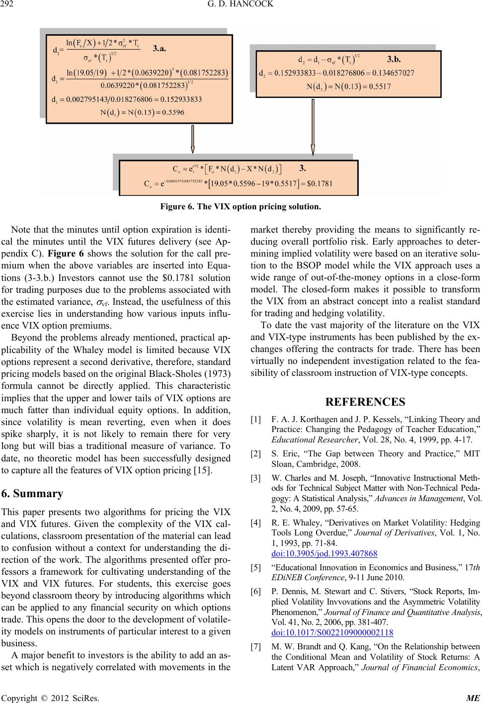

G. D. HANCOCK
292
Figure 6. The VIX option pricing solution.
Note that the minutes until option expiration is identi-
cal the minutes until the VIX futures delivery (see Ap-
pendix C). Figure 6 shows the solution for the call pre-
mium when the above variables are inserted into Equa-
tions (3-3.b.) Investors cannot use the $0.1781 solution
for trading purposes due to the problems associated with
the estimated variance, 
vf. Instead, the usefulness of this
exercise lies in understanding how various inputs influ-
ence VIX option premiums.
Beyond the problems already mentioned, practical ap-
plicability of the Whaley model is limited because VIX
options represent a second derivative, therefore, standard
pricing models based on the original Black-Sholes (1973)
formula cannot be directly applied. This characteristic
implies that the upper and lower tails of VIX options are
much fatter than individual equity options. In addition,
since volatility is mean reverting, even when it does
spike sharply, it is not likely to remain there for very
long but will bias a traditional measure of variance. To
date, no theoretic model has been successfully designed
to capture all the feature s of VI X opt ion pricing [15].
6. Summary
This paper presents two algorithms for pricing the VIX
and VIX futures. Given the complexity of the VIX cal-
culations, classroom presentation of the material can lead
to confusion without a context for understanding the di-
rection of the work. The algorithms presented offer pro-
fessors a framework for cultivating understanding of the
VIX and VIX futures. For students, this exercise goes
beyond classroom theory by introducing algorithms which
can be applied to any financial security on which options
trade. This opens the door to the development of volatile-
ity models on instruments of particular interest to a given
business.
A major benefit to investors is the ability to add an as-
set which is negatively correlated with movements in the
market thereby providing the means to significantly re-
ducing overall portfolio risk. Early approaches to deter-
mining implied vo latility were based on an iterative so lu-
tion to the BSOP model while the VIX approach uses a
wide range of out-of-the-money options in a close-form
model. The closed-form makes it possible to transform
the VIX from an abstract concept into a realist standard
for trading and hedging volatility.
To date the vast majority of the literature on the VIX
and VIX-type instruments has been published by the ex-
changes offering the contracts for trade. There has been
virtually no independent investigation related to the fea-
sibility of classroom instruction of VIX-typ e concepts.
REFERENCES
[1] F. A. J. Korthagen and J. P. Kessels, “Linking Theory and
Practice: Changing the Pedagogy of Teacher Education,”
Educational Researcher, Vol. 28, No. 4, 1999, pp. 4-17.
[2] S. Eric, “The Gap between Theory and Practice,” MIT
Sloan, Cambridge, 2008.
[3] W. Charles and M. Joseph, “Innovative Instructional Meth-
ods for Technical Subject Matter with Non-Technical Peda-
gogy: A Statistical Analysis,” Advances in Management, Vol.
2, No. 4, 2009, pp. 57-65.
[4] R. E. Whaley, “Derivatives on Market Volatility: Hedging
Tools Long Overdue,” Journal of Derivatives, Vol. 1, No.
1, 1993, pp. 71-84.
doi:10.3905/jod.1993.407868
[5] “Educational Innovation in Econ omics and Busine ss,” 17th
EDiNEB Conference, 9-11 June 2010.
[6] P. Dennis, M. Stewart and C. Stivers, “Stock Reports, Im-
plied Volatility Invvovations and the Asymmetric Volatility
Phenomenon,” Journal of Finance and Quantitative Analysis,
Vol. 41, No. 2, 2006, pp. 381-407.
doi:10.1017/S0022109000002118
[7] M. W. Brandt and Q. Kang, “On the Relationship between
the Conditional Mean and Volatility of Stock Returns: A
Latent VAR Approach,” Journal of Financial Economics,

G. D. HANCOCK 293
Vol. 72, No. 2, 2004, pp. 217-257.
doi:10.1016/j.jfineco.2002.06.001
[8] T. J. Ypma, “Historical Development of the Newton-Raph-
son Method,” SIAM Review, Vol. 37, No. 4, 1995, pp. 531-
551. doi:10.1137/1037125
[9] E. Derman and K. Iraj, “Riding the Smile,” Journal of Risk,
Vol. 7, No. 2, 1994, pp. 32-39.
[10] C. Corrado and S. Tie, “Skewness and Kurtosis in S&P
500 Index Returns Implied by Option Prices,” Journal of
Financial Research, Vol. 19, No. 2, 1996, pp. 175-192.
[11] I. Peña, G. Rubio and G. Serna, “Why do We Smile? On the
Determinants of the Implied Vola tility Function,” Journal of
Banking and Finance, Vol. 23, No. 8, 1999, pp. 1151-1179.
doi:10.1016/S0378-4266(98)00134-4
[12] F. Black and S. Myron, “The Pricing of Options and Cor-
porate Liabilities,” Journal of Political Economy, Vol. 81,
No. 3, 1973, pp. 637-654.
doi:10.1086/260062
[13] Z. G. Wang and D. Robe rt, “The Performance of VIX Op-
tion Pricing Models: Empirical Evidence beyond Simula-
tion,” Journal of Futures Markets, Vol. 31, No. 3, 2011, pp.
251-281.
[14] F. Black, “The Pricing of Commodity Contracts,” Journal
of Financial Economics, Vol. 3, No. 1-2, 1976, pp. 167-179.
doi:10.1016/0304-405X(76)90024-6
[15] Y. Lin and C. Chang, “VIX Option Pricing,” Journal of
Futures Market, Vol. 29, No. 6, 2009, pp. 523-543.
doi:10.1002/fut.20387

G. D. HANCOCK
294
Appendix A
S&P 500 ®index options contract specifications.
Symbol SPX
Underlying The Standard & Poor’s 500 cash Index.
Multiplier $100.
Premium Quote Stated in decimals. One point equals $100. Minimum tick for options trading below 3.00 is 0.05 ($5.00) and for all
other series, 0.10 ($10.00).
Strike Prices In-, at- and out-of-the-money strike prices are initially listed. New series are generally added when the underlying
trades through the highest or lowest strike price available.
Strike Price Intervals Five points. 25-point intervals for far months.
Expiration Date Saturday following the thir d Friday of the expiration month.
Exercise Style European—SPX options generally may be exercised only on the last business day before expiration.
Last Trading Day Trading in SPX options will ordinarily cease on the business day (usually a Thursday) preceding the day on which the
exercise-settlement value is calculated.
Settlement Value
Exercise will result in delivery of cash on the business day following expiration. The exercise-settlement value, SET,
is calculated using the opening sales price in the primary market of each component security on the last business day
(usually a Friday) before the expiration date. The exercise-settlement amount is equal to the difference between the
exercise-settlement value and the exercise price of the option, multiplied by $100.
Margin
Purchases of puts or calls with 9 months or less until expiration must be paid for in full. Writers of uncovered puts or
calls must deposit/maintain 100% of the option proceeds* plus 15% of the aggregate contract value (current index
level × $100) minus the amount by which the option is out-of-the-money, if any, subject to a minimum for calls of
option proceeds* plus 10% of the aggregate contract value and a minimum for puts of option proceeds* plus 10% of
the aggregate exercise price amount. (*For calculating maintenance margin, use option current market value instead of
option proceeds.) Additional m argin may be required pursuant to Exchange Ru l e 1 2 .1 0 .
Appendix B
VIX futures contract specifications.
Contract Name CBOE Volatility Index (VIX) Futures
Description The CBOE Volatility Index is based on real-time prices of options on the S&P 500 Index, listed on the Chicago Board Options Exchange (Symbol: SPX), and is designed to reflect investors’ consensus vi ew of future (30-day)
expected stock market volatility.
Contract Size $1000 times the VIX
No-Bust Range
CFE Rule 1202(l). The CFE error trade policy may only be invoked for 1) for trades executed during extended
trading hours for t he VIX futures contract, the E xcha nge error trade pol icy may only be invoked for a trade price
that is greater than 20% on either side of the market price of t he app lic ab le V IX fu tur e s c ont ra ct, a nd 2) fo r tr ade s
executed during regular trading hours for the VIX futures contract, the Exchange error trade policy may only be
invoked for a trade price that is greater than 10% on either side of the market price of the applicable VIX futures
contract. In accordance with Policy and Procedure III, the Help Desk will determine what the true market price for
the relevant Contract was imm ediately before the potential error trade occurred. In mak ing that determination, the
Help Desk may consider all relevant factors, including the last trade price for such Contract, a better bid or offer
price, a more recent price in a different contract month and the prices of related contr acts trading in other m arkets.
Termination of Trading The close of trading on the day before the Final Settlement Date. When the last trading d ay is m oved be cause of a CFE holiday, the last trading day for expiring VIX futures contracts will be the day immediately preceding the last
regularly-scheduled trading day.
Final Settlement Date
The Wednesday that is thirty days prior to the third Friday of the calendar month immediately following the
month in which the contract expires (“Final Settlement Date”). If the third Friday of the month subsequent to
expiration of the applicable VIX futures contr act is a CBOE holiday, the Final Settlement Date for the contract
shall be thirty days prior to the CBOE business day immediately proceeding that Friday.
Final Settlement Value
The final settleme nt value for VIX futures shal l be a Special Opening Quotati on (SOQ) of VIX calculated from the
sequence of opening prices of the opti ons used to calcula te the index on the settlement date. The opening price for
any series in which there is no trade shall be the average of that option's bid price and ask price as determined at
the opening of trading. The final se ttlement value will be rounded to the nearest $0.01. If the final settlement val ue
is not available or the normal settlement procedure canno t be utilize d due to a trading d isruptio n or other unus ual
circumstance, the final settlement value will be determined in accordance with the rules and bylaws of The
Options Clearing Corporation.
Delivery Settlement of VIX futures contracts will result in the delivery of a cash settlement amount on the business day
immediately following the Final Settlement Date. The cash settlement amount on the Final Settlement Date shall
be the final mark to marke t amount against the final settlement value o f t h e VIX futures multiplied by $1000.00.
Source: CBOE Delayed Quotations.