ABSTRACT

This paper presents the theory and applications of a new computational technique referred to as Differential Transform Method (DTM) for solving second order linear ordinary differential equations, for both homogeneous and nonhomogeneous cases. For the robustness and efficiency of the method, four examples are considered. The results indicate that the DTM is reliable and accurate when compared to the exact solutions of the solved problems.

Keywords:Differential Transform Method, Second Order ODEs, Linear Systems, Series Solution

1. Introduction

Most of the problems encountered in applied sciences, management and economics take the forms of second order linear ordinary differential equations. Sometimes, obtaining exact solutions through the direct methods (analytical methods) for these systems seems difficult even if the exact solutions exist, hence the need for numerical techniques for approximate solutions. Some of these numerical methods involve linearization, disscretization and perturbation, and they only permit the solutions to a given ODE at a certain interval. In addition, they are intensive in terms of computation and as such, lead to the situations where some basic phenomena are technically avoided.

The notion of DTM was first introduced by Zhou [1] while solving linear and nonlinear initial value problems in electric circuit analysis. The Method provides an analytical approximate solution to linear and nonlinear systems of differential equations. This involves the construction of a semi-analytical technique with the aid of a Taylor series expansion for the solutions in polynomial forms. The DTM has been proven by many researchers [1] -[7] to be very effective and efficient in handling differential equations with point boundary value problems, kvd and mkdv differential-algebraic equations, and so on. It also reduces the size of computational work while maintaining high accuracy even with a fast convergence rate compared to the theoritical solutions [8] .

Some other analytical methods like the variational iterative method and the Adomian decomposition method witness difficulties in handling functions involving complicated integrals; since successive component using those methods depends on the previous component [9] -[13] but DTM overcomes this by solving an algebraic recursive equation.

2. The Differential Transform Method

This section introduces the basic concepts and theorems of DTM needed for applications in the remaining sections.

Definition 1. Let be a given function of one variabe defined at a point, then the one-dimensional differential transform of the defined as is given as:

(1)

Equation (1) is the transformed function of.

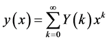
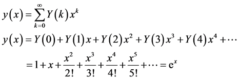
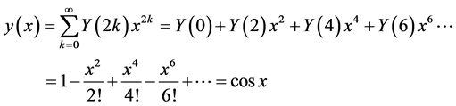
Definition 2. The differential inverse transform of is a Taylor series expansion of the function about, defined as :

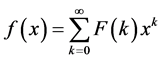(2)

Combining (1) and (2) yields:

(3)

2.1. Some Basic Theorems of the Differential Transform Method

The following theorems and properties of the DTM are stated below for the sake of applications, their proofs can be found in [14] and [15] .

Let, and be differentiable functions with differential transforms, and respectively, with, and a Kronecker delta, then the following theorems hold:

Theorem 2.1 If then

Theorem 2.2 If then

Theorem 2.3 If then such that:

Theorem 2.4 If then, where α is a constant.

Theorem 2.5 If then.

In particular, we have:

(a) If then

(b) If then

2.2. The DTM and the Second order Linear Ordinary Differential Equations (ODEs)

In this section, we present clearly how a second order linear ODE with constant coefficients is transformed using the DTM.

The corresponding ODE is of the form:

(4)

with initial conditions and

Equation (4) is re-expressed in the form of

(5)

Thus, (4) becomes

(6)

We will take the differential transform (DT) of (6) by applying theorems (2.1-2.6) as follows:

(7)

(8)

(9)

subject to the initial conditions.

Equation (9) is a recursive formula for the computation of coefficient terms in the series solution of the problem. Therefore, using (2) and (9) gives the approximate solution of (4) as:

(10)

3. Applications and Numerical Results

In this section, we will apply the discussed DTM to solve some problems whose results will be compared with the theoretical (exact) solutions. Two cases with two examples each are considered. Case I and Case II for homogeneous and nonhomogeneous respectively.

Case I Example 1: Consider the ODE

(11)

subject to, with a theoretical solution

(12)

Procedure We rewrite (11) in a standard form and take the differential transform (DT) as follows:

(13)

(14)

(15)

with the initial conditions.

By using the recursive relation in (15) with, we obtain values for, as showed below:

For; for; for; for,; for

But from (10),

(16)

Equation (16) is the same with the theoretical solution in (12).

Case I Example 2: Consider the ODE

(17)

subject to, with a theoretical solution

(18)

Procedure We re-write (16) in a standard form and take the differential transform as follows:

(19)

with the initial conditions.

Computing using (19) gives the following:

For; for; for; for, for,; for

We observed that. Hence, the solution of (17) by (10) is reformed as:

(20)

Equation (20) agrees with the theoritical solution in (18).

Case II Example 1: Consider the ODE

(21)

subject to, with a theoretical solution:

(22)

Procedure Equation (21) by the differential transform method becomes;

(23)

with the initial conditions.

Thus, for, the values of, obtained using (23) are given below:

For; for; for; for, for; for.

As such, from (10), the solution of (21) is:

(24)

Since

(25)

(26)

Equation (26) is the same with the theoretical solution in (22).

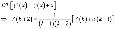
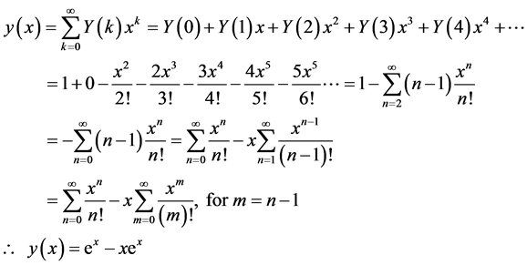
Case II Example 2: Consider the ODE

(27)

subject to, with a theoretical solution:

(28)

Procedure Equation (27) by the differential transform method becomes;

(29)

subject to the initials.

Thus, for, the values of, obtained using (29) are given below:

For; for; for; for, for ;; for.

Hence, from (10), the solution of (27) is:

(30)

Equation (30) corresponds with the theoretical solution in (28).

Remark 3.1:

We present numerical comparisons between the exact, and the numerical solutions based on a 5-iterate DTM using the coefficient terms from Table 1, Table 2, Table 3, and Table 4 as shown in Table 5, Table 6, Table 7, and Table 8 respectively.

4. Discussion of Results and Conclusion

In this paper, we have presented a semi-analytical method (DTM) for solving a certain class of ODEs. The DTM has advantages over other numerical techniques as it does not involve linearization, discretization or perturbation of a given problem; hence it has no effect of computational round off error. The DTM also provides a closed-form solution; therefore, it is very powerful and effective in finding both analytical and numerical solutions of second order linear ODEs with constant coefficients.

References

NOTES

^*Corresponding author.

References

- Zhou, J.K. (1986) Differential Transformation and its Applications for Electrical Circuits. Huazhong University Press, Wuhan.
- Chen, C.L. and Liu, Y.C. (1988) Solution of Two Point Boundary Value Problems Using the Differential Transformation Method. Journal of Optimization Theory and Applications, 99, 23-35. http://dx.doi.org/10.1023/A:1021791909142
- Ayaz, F. (2004) Application of Differential Transform Method to Differential-algebraic Equations. Applied Mathematics and Computation, 152, 649-657. http://dx.doi.org/10.1016/S0096-3003(03)00581-2
- Kangalgil, F. and Ayaz, F. (2009) Solitary Wave Solutions for the kdv and mkdv Equations by Differential Transform Method. Chaos, Solitons and Fractals, 41, 464-472. http://dx.doi.org/10.1016/j.chaos.2008.02.009
- Batiha, K. and Batiha, B. (2011) A New Algorithm for Solving Linear Ordinary Differential Equations. World Applied Sciences Journal, 15, 1774-1779.
- Thongmoon, M. and Pusjuso, S. (2010) The Numerical Solutions of Differential Transform Method and the Laplace Transform Methods for a System of Differential Equations. Nonlinear Analysis: Hybrid Systems, 4, 425-431. http://dx.doi.org/10.1016/j.nahs.2009.10.006www.elsevier.com/locate/nahs
- Ravi Kanth, A.S.V. and Aruna, K. (2009) Differential Transform Method for Solving the Linear and Nonlinear Klein-Gordon Equation. Computer Physics Commmunications, 180, 708-711. http://dx.doi.org/10.1016/j.cpc.2008.11.012
- Chang, S.H. and Chang, I.L. (2008) A New Algorithm for Calculating One-Dimensional Differential Transform of Nonlinear Functions. Applied Mathematics and Computation, 195, 799-808. http://dx.doi.org/10.1016/j.amc.2007.05.026
- Adomian, G. (1994) Solving Frontier Problems of Physics. The Decomposition Method. Springer, New York.
- Ibijola, E.A. and Adegboyegan, B.J. (2008) On the Theory and Application of Adomian Decomposition Method for Solution of Second Order ODEs. Pacific Journal of Science and Technology, 9, 357-362.
- Shousa, D.-H. and He, J.-H. (2008) Beyond Adomian Method: The Variational Iteration Method for Solving Heat-Like and Wave-Like Equations with Variable Coefficients. Physics Letters A, 372, 233-237. http://dx.doi.org/10.1016/j.physleta.2007.07.011
- He, J.-H. (2007) Variational Iterative Method—Some Recent Results and New Interpretations. Journal of Computational and Applied Mathematics, 207, 3-17. http://dx.doi.org/10.1016/j.cam.2006.07.009
- Catal, S. (2012) Some of Semi Analitical Methods for Blasius Problem. Applied Mathematics, 3, 727-728. http://dx.doi.org/10.4236/am.2012.37106
- Arikoglu, A. and Ozkol, I. (2005) Solution of Boundary Value Problems for Integro-Differential Equations by Using Transform Method. Applied Mathematics and Computation, 168, 1145-1158. http://dx.doi.org/10.1016/j.amc.2004.10.009
- Odibat, Z. (2008) Differential Transform Methods for Solving Volterra Integral Equations with Separable Kernels. Mathematical and Computer Modelling, 48, 1144-1146. http://dx.doi.org/10.1016/j.mcm.2007.12.022