Open Journal of Marine Science, 2012, 2, 58-65
http://dx.doi.org/10.4236/ojms.2012.22008 Published Online April 2012 (http://www.SciRP.org/journal/ojms)
Spatial and Temporal Features of Regional Variations in
Mean Sea Level around Taiwan
Li-Chung Wu1, Chia Chuen Kao2, Tai-Wen Hsu2*, Yi-Fung Wang3, Jong-Hao Wang3
1Coastal Ocean Monitoring Center, National Cheng Kung University, Tainan, Chinese Taipei
2Department of Hydraulic and Ocean Engineering, National Cheng Kung University, Tainan, Chinese Taipei
3Water Resources Agency, Ministry of Economic Affairs, Taip e i, Chinese Taipei
Received January 10, 2012; revised March 9, 2012; accepted March 18, 2012
ABSTRACT
Satellite altimeter and in-situ tide gauge record s are probably the most common means to obtain observational data for
the study of changes in mean sea level. In this study, we employed these data to discuss the spatial and temporal fea-
tures of regional variations in mean sea level around Taiwan. The results showed that most of the regional mean sea
surface heights (SSH) around Taiwan are higher than the global mean sea surface heights. Most of the sea level trends
are greater than the global mean sea level trend as well. We obtained diverse distribution results from the altimeter sea
level records in neighboring areas by distributions fit, and the altimeter sea level records showed obv ious inhomogene-
ity. In addition, periodic f luctuations in the record s regarding mean sea level were revealed in our study, based on Fou-
rier spectra and wavelet scalograms.
Keywords: Sea Level Variations; Tide-Gauge; Altimeter
1. Introduction
The United Nations estimates that by 2004, more than
75% of the world’s population was living within the
coastal zone, and th e importance of these region s extend s
to their influence on global economic activities [1]. Be-
cause several million people liv e in coastal areas that are
less than 10 meters above sea level, the features of sea
level are a critical factor in the development of human-
kind. Sea levels fluctuate due to natural phenomena, such
as wind waves, swell, tsunamis, astronomical tides, storm
surges, and other various factors. In addition, atmos-
pheric pressure, ocean currents, and changes in local
ocean temperatures can also influence variations in mean
sea level. In recent years, thermal expansion of the
oceans was expected to be a dominant factor behind in-
creases in sea level [2]. For extremely mild slope coastal
areas, even a small increase in sea level could result in a
serious threat to coastal environments. Indications of
global warming revealed through various atmospheric
and oceanic records are pushing the discussion of long-
term changes in sea levels to the forefront of the global
research community.
Taiwan is an island located at the western edge of the
Pacific Ocean, lying on the border between the largest
land mass and the largest ocean in the world. The coast-
line around Taiwan covers a total length of over one
thousand kilometers, and the surrounding bathymetry is
highly complicated. Along the east coast of Taiwan, the
seafloor drops rapidly to thousands of meter in depth
from the coastline, with a slope in this area of approxi-
mately 1/10. Compared to the eastern Taiwan, the slope
(about 1/100 - 1/50) along the west coast is relatively
mild. In some areas of west coast, the slope can be milder
than 1/1500. Due to the potential impact on the coastal
environment, understanding the features of sea level va-
riation around Taiwan is an issu e of great concern.
This study focuses on the phenomenon of long-term
variations in sea level and in-situ sea level records from
coastal tide stations are ideally suited to such research.
Church and White [3] poin ted that g loba l mean sea lev els
have risen an average of approximately 1.7 mm/year and
a significant acceleration in the rise of sea-levels of ap-
proximately 0.013 mm/year2. To accurately evaluate the
rate of change in sea levels, the effects of tectonic
movements or local subsidence upon the measurement of
mean sea level has to be taken into consideration. It is
essential to adjust perceived ch anges in mean sea level to
account for vertical movements of the land, which may
be of the same order as changes in the sea level around
Taiwan or even higher [4]. However, most of the bench-
mark tide gauges were not corrected in the former time
and the actual magnitude of land subsidence was practi-
*Corresponding a uthor.
C
opyright © 2012 SciRes. OJMS

L.-C. WU ET AL. 59
cally unknown. It is difficult to identify trends in the
changes of sea levels using uncorrected tide gauge re-
cords. Since the 1990s, satellite altimetry has provided
most of the information regarding regional sea levels
both in Taiwan and globally. Satellite altimetry deter-
mines the distance from the satellite to the surface of the
sea by measuring the satellite-to-surface round-trip time
of a radar pulses. Previous studies presented changes in
global mean sea levels based on the Topex-Poseidon
altimetry data [5,6].
A large number of studies have revealed the features
of global sea level chang e by discussing altimeter records;
however, the issue of regional sea level characteristics
has received little attention. With respect to the land,
mean sea level is a relatively stable surface value; how-
ever, it varies irregularly in the time and space domain.
The aim of this study was to discuss the spatial and tem-
poral features of variations in regional sea levels around
Taiwan. Results of statistical and spectral analysis are
presented in our study, to confirm the local features of
sea level variation in Taiwanese waters.
2. Data Source
Satellite altimeter and in-situ tide gauge records are
probably the most common means to obtain observa-
tional data for the study of changes in mean sea level.
White et al. [7] used satellite and in-situ data to discuss
coastal and global averaged sea level rise. In our study,
we focus on the local features of sea level around Taiwan.
To evaluate the spatial features of sea levels in Taiwan-
ese waters, we used altimeter data from the merged geo-
physical data (MGDRB) records. The altimeter products
were produced by Ssalto/Duacs and distributed by Aviso
[8]. Sea level anomalies (SLA) describe variations in sea
surface height (SSH) with respect to a mean sea surface
(MSS). The SSH is the height of the sea surface with
respect to a reference ellipsoid, and MSS information
provides the ocean surface averaged vertical position
over a period of time. The spatial resolution of SLA was
resampled on a 1/4˚ × 1/4˚ Cartesian grid. In addition to
the spatial resolution, temporal resolution had to be con-
sidered. The temporal resolution of SLA from the al-
timeter record was 7 days. To obtain accurate sea level
data, the influence of atmosphere and ionosphere upon
the velocity of altimeter radio pulses also had to be con-
sidered. The sea level data from Aviso had already been
corrected by propagation, ocean surface, and geophysical
and atmospheric corrections. Error due to the atmosphere
through which the radar pulse travels and the nature of
the reflecting surface also had to be corrected.
The data used in our analysis comprised more than 15
years of altimetry data (1993-2008). The selection of
spatial altimeter records around Taiwan is shown in Fig-
ure 1. Because the west coast of Taiwan is a 200-km-
wide shallow passage, it is impossible to select a large
area that is not affected by the edges of Mainland China
or Taiwan. Here we selected nine grids in each local area
of the sea. These nine grids were arrayed as a 3 × 3 ma-
trix, to address the spatial features of altimeter records
from neighboring grids. Four different record matrices
were selected from the sea areas around Taiwan. Because
these four matrices are located north, east, west, and
south of Taiwan, these matrices were named MN, ME,
MW, and MS in the following sections. In addition, the
sea level data from four different in-situ tide stations
(Keelung, Fugang, Taichung, and Xunguangzui) was also
collected in this study. It should be noted that the loca-
tions of these in-situ tide stations was close to altimeter
record matrices. To obtain accurate sea level information,
the effects of surface atmospheric pressure on low fre-
quency sea level variability had to be removed [9]. The
altimeter records were corrected by the ECMWF model.
The in-situ sea surface data from four different in-situ
tide stations were corrected by the in-situ air pressure
data, this method was proposed by Wunsch and Stammer
[10].
3. Data Analysis
3.1. Statistical Features of Regional Sea Level
Figure 2 presents altimeter sea level data observed in
several areas of the sea. It appears that the sea levels are
increasing in these areas. As previously mentioned, we
selected nine grids from the altimeter records in each
local sea area. These nine grids were arrayed as a 3 × 3
Figure 1. Locations of data sets obtained from altimeter and
n-situ tide stations. i

L.-C. WU ET AL.
60
Figure 2. Sea level records from altimeter data.
matrix, the location (I, J) indicates the element at the I-th
row and the J-th column. The rate of change in the sea
level calculated in different areas is presented in Figure
3, revealing that increases in sea level in the same area
were uniform. However, differences in sea level rise
rates in various areas around Taiwan can be as high as 5
mm/year. This indicates obvious spatial inhomogeneity
in the altimeter records among various regions of the sea
around Taiwan. Homogeneity means that the statistical
properties do not change with space; and inhomogeneity
implies instability in the statistical p roperties of th e space
domain. Figure 3 also presents calculated sea level trends
from in-situ tide gauge records. Because the in-situ tide
stations at Keelung, Fugang, Taichung, and Xunguangzui
are close to the sea areas of MN, ME, MW, and MS re-
spectively, we used the same designations to present the
results from the in-situ data in Figure 3.
Regardless of the results from altimeter or tide gauge
records, most of the calculated results of regional sea
level trends exceeded 4 mm/year. Church and White [3]
revealed the global average rate of mean sea levels ana-
lyzed from in-situ tide records (data records from 1870 to
2004), estimating the increase at 1.7 mm/year. Ablain et
al. [11] presented the global mean sea level rate from
altimeter records (data records from 1993 to 2009), esti-
mated at 3.26 mm/year. The increase in the rate of re-
gional sea level trends around Taiwan is greater than
global mean sea level trends.
The in-situ records from tide stations in the western
and northern parts of Taiwan showed results similar to
those calculated from altimeter records. However, the
results from eastern and southern in-situ records did not
match the results from the altimeter records. In the
southern sea area of Taiwan, land subsidence may have
been one contributing factor. According to a report from
the Taiwanese government [12], the south-west coastal
area is one area with the greatest subsidence in Taiwan,
due to over use of the lo cal ground water. The maximum
accumulated subsidence has been as high as 2.88 m since
1972. Essentially, the influences of subsidence on the
bench mark are unavoidable. In addition to the south-
west coastal area, the east coast of Taiwan is one of the
most actively deforming regions in the world. Yu and
Kuo [13] presented evidence of land surface uplift
through repeated GPS readings. This is one probable
reason that the calculated rate of change in sea levels is
lower than the actual rate in the eastern part of Taiwan.
From the time series shown in Figure 2, we observe ob-
vious fluctuations in sea level along the west coast of
Taiwan. Figure 4 shows the standard deviation in sea
level records from various sea areas. The values of stan-
dard deviation calculated fro different sea areas have m

L.-C. WU ET AL. 61
Figure 3. Trends of sea level change around Taiwan.
Figure 4. Standard deviation in sea level records.
also shown obvious inhomogeneity, with the values of
MW exceeding those in other sea areas. It should be noted
that tidal differences within the Taiwan Strait are larger
than other areas around Taiwan. The influence of such
obvious tidal differences is a likely reason for the varia-
tions in sea level in the area of MW. For the relationship
between the results of standard deviation from in-situ
observation and remote sensing, the other cases showed
similarities in all of the values of calculated standard
deviation between altimeter and in-situ tide gauge re-
cords except for those in eastern Taiwan.
3.2. The Distributions of Mean Sea Level
Records
Probability distribution based on the stochastic process
provides a key to evaluating various characteristics o f sea
level. The distribution functions of Beta, Normal, Chi-
squared, Log-gamma, Logistic, Rayleight, Weibull, Gen-
erated Extreme Values were used to determine the ideal
distribution in every sea level time series. We employed
the chi-squared test for the goodness of fit. Dep ending on
the chosen goodness of fit tests, we calculated the chi-
squared test for each of the fitted distributions. If the
chi-squared test were unable to reject impractical distri-
bution functions, the minimal differences between the
selected distribution function and the distribution of sea
level data would be used to determine the distribution
function with the best fit. Table 1 presents the fitted dis-
tribution functions of sea level records. Most of the sea
level records from various in-situ tide stations showed
Generalized Extreme Value distributions. However, we
often obtained different distributions from the altimeter
records within the matrix in the same sea areas, particu-
larly for those within MW. We obtained five different
distribution functions from nine elements of MW. The
results of distribution fitness once again showed spatial
non-homogeneity of altimeter sea level records. We
evaluated the mean, skewed values of various distribu-
tions fitted from the time series of sea level records. In
Figure 5, the value of zero on the y-axis indicated the
sea surface height averaged across all the oceans of the
globe. Figure 5 illustrates that most of the sea surface
heights observed around Taiwan were higher than the
global mean surface height. The records from the east
coast of Taiwan showed higher sea surface height than
the records from other sea areas. The regional sea surface
height along the south coast of Taiwan was closer to the

L.-C. WU ET AL.
62
global mean. Because the benchmarks between altimeter
and in-situ tide records were different, the mean values
of in-situ records are not presented in Figure 5. Figure 6
shows that most of the calculated skewness values from
MN and MS were close to zero, indicating that sea surface
height distribution in these two sea areas was more sym-
metric. However, the distribution of sea surface height in
the east sea area showed obvious negative skewness.
3.3. Spectral Features
As shown in Figure 2, we observed complicated os cilla-
tions in all-time series of sea level records. To reveal
these oscillations, we applied a spectrum to analyze sea
level records. Figure 7 presents the Fourier spectra ana-
lyzed from a variety of altimeter and tide gauge records,
revealing the peak frequency of 1 year–1 compr i s i n g mo s t
of the sea level records. The fluctuations in sea level
were probably influenced by the inverted barometer,
even though the altimeter and in-situ sea level records
had already been corrected by the ECMWF model and
in-situ barometric pressure data, respectively. In addition,
the temperature of sea water is likely another main factor
Table 1. Distribution of sea level data.
MN M
E M W M S
(1, 1) Normal Beta Logistic Beta
(1, 2) Weibull (3P) Beta Beta Normal
(1, 3) Normal Beta Gen. Extreme ValueBeta
(2, 1) Normal Beta Logistic Normal
(2, 2) Weibull (3P) Normal Normal Normal
(2, 3) Weibull (3P) Beta Beta Normal
(3, 1) Weibull (3P) Beta Normal Beta
(3, 2) Weibull (3P) Normal Normal Gen. Extreme Value
(3, 3) Normal Beta We ibu ll (3P ) Normal
Tide station Gen. Extreme ValueGen. Ex treme ValueWeibull (3P) Gen. Extreme Value
Figure 5. Mean of sea level records.
Figure 6. Skewness of sea level distribution.

L.-C. WU ET AL. 63
Figure 7. Fourier spectra of sea level data.
influencing the oscillation of sea level. Both air pressure
and sea temperature have one year oscillatio ns due to the
influences of the seasons. The spectra in Figure 7 also
show energy density in some higher frequency bands.
The energy density of some astronomical tide constitu-
ents can be observed from the Fourier spectra of MW, MN
and MS, including the lunar monthly constituents (Period
= 13.2 year) and luni-solar fortnightly constituents (Pe-
riod = 24.7 year). Unlike the other sea areas, the spectra
from ME did not show obvious energy density from the
higher frequency band. From most of the Fourier spectra
obtained in Taiwan waters, we observed strong energy
density located around the frequency bands of 6 year–1
and 0.1 year–1. This study revealed the bi-monthly and
ten-year oscillations of the sea level. In addition to the
Fourier spectrum, we investigated non-stationary features
of sea level time series by wavelet scalogram. Wavelet
transform is similar to Fourier transform in that it breaks
signals into their constituents. However, the wavelet
scalogram provides extra resolution to the signal energy
in the time domain as well as the frequency domain. It is
a useful tool for determining the oscillation of sea level
records both in the time and frequency domain simulta-
neously. To implement the wavelet algorithm, it is nec-
essary to choose a mother wavelet function first. We se-
lected the Morlet wavelet function, commonly used in
spectrum analysis [14,15], to identify sea surface infor-
mation from the altimeter records. It should be men-
tioned that the wavelet scalogram presents the time-fre-
quency variations of spectral components, but at a dif-
ferent time-frequency resolution. For the low frequency
information from the wavelet scalogram, the time resolu-
tion is poor but frequency resolution is high. When it is
shifted toward high frequencies, the time resolution in-
creases but the frequency resolution decreases. This is
very similar to the Heisenberg Uncertainty Principle [16].
We obtained various results from the wavelet scalogram
for each element of the altimeter matrix. In other words,
36 different scalogram results were calculated from four
different sea areas around Taiwan. The features of wave-
let scalograms from the nine elements of each altimeter
record matrix were similar. We averaged the sea level
records from nine grids of each matrix. Based on the re-
sults of wavelet scalograms from various sea areas (Fig-
ure 8), we revealed the non-stationarity in the time series
of the altimeter records. The energy density in the fre-
quency band of 1 year–1 did not stabilize within the entire
time domain. For the results from northern sea areas, the
1-year oscillation was more obvious during 1997-1999
and 2002-2005 than that during other years. It should be
noted that the 1-year oscillations in different sea areas
were dissimilar. Compared to the results from Fourier
spectra, we observed clear energy density from the high
frequency bands of the wavelet scalogram. The distribu-
tion of high frequency energy density was also non-sta-
tionary. Most of the high frequency energy density oc-
curred in the summer and autumn. Similar to the results
from the Fourier spectrum, we also observed the energy
of lunar monthly constituents (Period = 13.2 year) from
the wavelet scalogram of different sea areas. However,

L.-C. WU ET AL.
64
the energy density in the frequ ency band did no t stabilize
within the entire time domain. We applied the non-sta-
tionarity index, to verify and determine the degree of the
non-stationarity from different kinds of time series of sea
level records. The theory behind the non-stationarity in-
dex was proposed by Liu [17], based on the wavelet sca-
logram. The non-stationarity Index (NI) was defined as:

 

2
,
Iiji
ij
NWftff
 i
(1)
 
1,
T
iij
j
f
Wft T






(2)
where W(fi, tj) is the wavelet scalogram, fi is the fre-
quency bins, tj is the time, T is the total number of data
points. Based on Equation (1) and Equation (2), a time
series with a larger NI is likely to be more non-stationary
than ones whose NI is smaller. Figure 9 presents the cal-
culated results of the non-stationarity index from the sea
level records in different sea areas. The longer the sea
level records were, the higher of the non-stationarity in-
dex was. Figure 9 also shows that the results of the non-
stationarity index were higher in the sea area of ME and
lower in the sea area of MW. Figure 9 reveals that the
oscillations of sea level within the sea area of MW were
more stationary than in other sea areas.
4. Conclusions
The trends associated with changes in sea level have
been a topic of particular concern since scientists first
noticed signs of global warming. Due to obvious differ-
ences in bathymetry between the west and east coasts of
Taiwan, understanding the regional sea level patterns
around the island is essential to characterizing the phe-
nomenon of sea level chang e. This study investigated the
statistical and spectral characteristics of sea level in the
Figure 8. Wavelet scalogram from altimeter data.
Figure 9. Non-stationarity index calculated from altimeter records.

L.-C. WU ET AL. 65
regional sea areas around Taiwan, through the analysis of
in-situ tide gauge and satellite altimetry records. After
calculating the sea level tren ds from the altimetry record s,
we revealed similarities in the rates associated with sea
level trends calculated in the same sea area. However,
differences in the trends of sea level change calculated in
different sea areas around Taiwan can be as high as 5
mm/year.
In addition, sea surface heights around Taiwan are
higher than the global mean surface height. It should also
be noted that the calculated results between in-situ and
altimeter records were quite different in some sea areas
around Taiwan. Subsidence and land surface uplift no
doubt have a significant influence on the accuracy of
calculated sea level trends. We also discussed the prob-
ability distribution of sea level records. The results of
distribution fitness showed spatial inhomogeneity of sea
level records, and differences in the distribution from
altimeter time series within the same matrix, particularly
in the west sea area of Taiwan.
To reveal the fluctuations in sea level records, we em-
ployed various tools incorporating spectral transform.
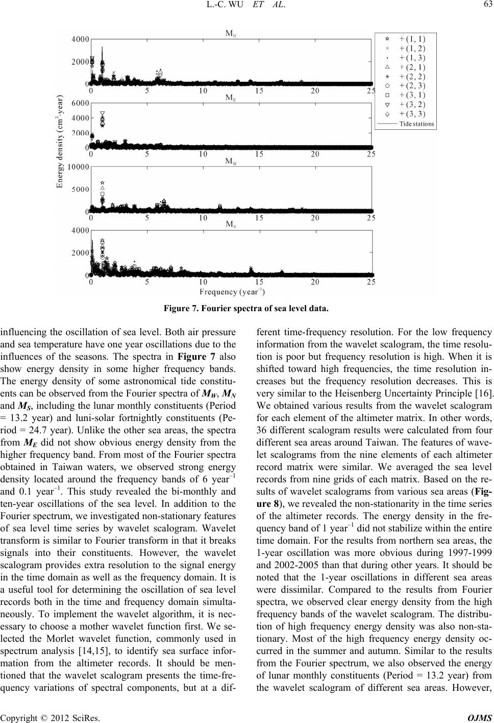
From the results of Fourier spectra, we confirmed a num-
ber of obvious fluctuations in the sea level records. An-
nual fluctuations in most of the sea level records from
altimeter and in-situ tide gauge records were quite obvi-
ous, and a few of the astronomical tide con stituents were
observed in the Fourier spectra. In addition to the Fo urier
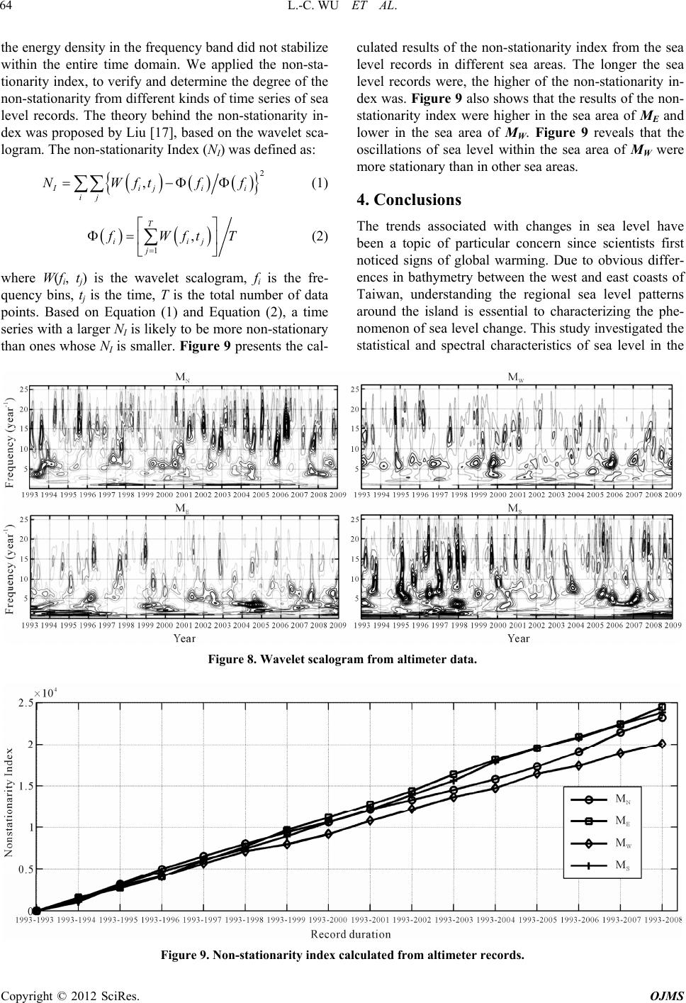
spectra, we discussed the non-stationary features of sea
level time series according to wavelet scalograms. The
energy density from various frequency bands showed
non-stationarity in the time series of altimeter records.
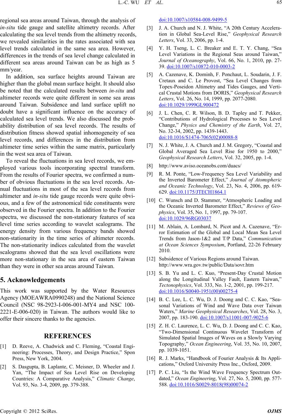
The non-stationarity indices calculated from the wavelet
scalograms showed that the sea level oscillations were
more non-stationary in the sea area of eastern Taiwan
than they were in other sea areas around Taiwan.
5. Acknowledgements
This work was supported by the Water Resources
Agency (MOEAW RA0990248) and the Nation al Science
Council (NSC 98-2923-I-006-001-MY4 and NSC 100-
2221-E-006-020) in Taiwan. The authors would like to
offer their sincere thanks to the agencies.
REFERENCES
[1] D. Reeve, A. Chadwick and C. Fleming, “Coastal Engi-
neering: Processes, Theory, and Design Practice,” Spon
Press, New York, 2004.
[2] S. Dasgupta, B. Laplante, C. Meisner, D. Wheeler and J.
Yan, “The Impact of Sea Level Rise on Developing
Countries: A Comparative Analysis,” Climatic Change,
Vol. 93, No. 3-4, 2009, pp. 379-388.
doi:10.1007/s10584-008-9499-5
[3] J. A. Church and N. J. White, “A 20th Century Accelera-
tion in Global Sea-Level Rise,” Geophysical Research
Letters, Vol. 33, 2006, pp. 1-4.
[4] Y. H. Tseng, L. C. Breaker and E. T. Y. Chang, “Sea
Level Variations in the Regional Seas around Taiwan,”
Journal of Oceanography, Vol. 66, No. 1, 2010, pp. 27-
39. doi:10.1007/s10872-010-0003-2
[5] A. Cazenave, K. Dominh, F. Ponchaut, L. Soudarin, J. F.
Cretaux and C. Le Provost, “Sea Level Changes from
Topex-Poseidon Altimetry and Tides Gauges, and Verti-
cal Crustal Motions from DORIS,” Geophysical Research
Letters, Vol. 26, No. 14, 1999, pp. 2077-2080.
doi:10.1029/1999GL900472
[6] J. L. Chen, C. R. Wilson, B. D. Tapley and T. Pekker,
“Contributions of Hydrological Processes to Sea Level
Change,” Physics and Chemistry of the Earth, Vol. 27,
No. 32-34, 2002, pp. 1439-1443.
doi:10.1016/S1474-7065(02)00088-8
[7] N. J. White, J. A. Church and J. M. Gregory, “Coastal and
Global Averaged Sea Level Rise for 1950 to 2000,”
Geophysical Research Letters, Vol. 32, 2005, pp. 1-4.
[8] http://www.aviso.oceanobs.com/duacs/
[9] R. M. Ponte, “Low-Frequency Sea Level Variability and
the Inverted Barometer Effect,” Journal of Atomspheric
and Oceanic Technology, Vol. 23, No. 4, 2006, pp. 619-
629. doi:10.1175/JTECH1864.1
[10] C. Wunsch and D. Stammer, “Atmospheric Loading and
the Oceanic Inverted Barometer Effect,” Reviews of Geo-
physics, Vol. 35, No. 1, 1997, pp. 79-107.
doi:10.1029/96RG03037
[11] M. Ablain, A. Lombard, N. Picot and A. Cazenave, “Er-
ror Estimation of the Global and Local Mean Sea Level
Trends from Jason-1&2 and T/P Data,” Communication
at Ocean Sciences Symposium, Portland, 22-26 February
2010.
[12] Subsidence of Various Regions around Taiwan.
http://www.wra.gov.tw/public/Data/sovr.htm
[13] S. B. Yu and L. C. Kuo, “Present-Day Crustal Motion
along the Longitudinal Valley Fault, Eastern Taiwan,”
Tectonophysics, Vol. 333, No. 1-2, 2001, pp. 199-217.
doi:10.1016/S0040-1951(00)00275-4
[14] B. C. Lee, L. C. Wu, D. J. Doong and C. C. Kao, “Sea-
sonal Variations of Wind and Wave Data over Taiwan
Waters,” Marine Geophysical Researches, Vol. 28, No. 3,
2007, pp. 183-190. doi:10.1007/s11001-007-9025-6
[15] Z. H. C. Laurence, L. C. Wu, D. J. Doong and C. C. Kao,
“Two-Dimensional Continuous Wavelet Transform of
Simulated Spatial Images of Waves on a Slowly Varying
Topography,” Ocean Engineering, Vol. 35, No. 10, 2007,
pp. 1039-1051.
[16] R. J. Marks, “Handbook of Fourier Analysis & Its Appli-
cations,” Oxford University Press Inc., Oxford, 2009.
[17] P. C. Liu, “Is the Wind Wave Frequency Spectrum Out-
dated,” Ocean E ngineering, Vol. 27, No. 5, 2000, pp. 577-
588. doi:10.1016/S0029-8018(98)00074-2