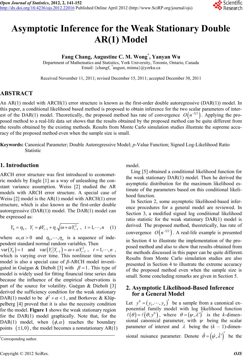Open Journal of Statistics, 2012, 2, 141-152
http://dx.doi.org/10.4236/ojs.2012.22016 Published Online April 2012 (http://www.SciRP.org/journal/ojs) 141
Asymptotic Inference for the Weak Stationary Double
AR(1) Model
Fang Chang, Augustine C. M. Wong*, Yanyan Wu
Department of Mathematics and Statistics, York University, Toronto, Ontario, Canada
Received November 11, 2011; revised December 15, 2011; accepted December 30, 2011
ABSTRACT
An AR(1) model with ARCH(1) error structure is known as the first-order double autoregressive (DAR(1)) model. In
this paper, a conditio nal likelihood based meth od is proposed to obtain inferen ce for the two scalar parameters of inter-
est of the DAR(1) model. Theoretically, the proposed method has rate of convergence

32
On
. Applying the pro-
posed method to a real-life data set shows that the results obtained by the proposed method can be quite different from
the results obtained by the existing methods. Results from Monte Carlo simulation studies illustrate the supreme accu-
racy of the proposed method even when the sample size is small.
Keywords: Canonical Parameter; Double Autoregressive Model; p-Value Function; Signed Log-Likelihood Ratio
Statistic
1. Introduction
ARCH error structure was first introduced to economet-
ric models by Engle [1] as a way of unleashing the con-
stant variance assumption. Weiss [2] studied the AR
models with ARCH error structure. A special case of
Weiss [2] model is the AR(1) model with ARCH(1) error
structure, which is also known as the first-order double
autoregressive (DAR(1)) model. The DAR(1) model can
be expressed as:
00
Y

, 21t t
Y 

1, ,tn
1tt
YY   , (1)
where ,0

  and 0n ,,

 
r
is a sequence of inde-
pendent standard normal random variables. Then
and

0
Yva 1

2
var YY Y   1, ,tn
11tt t
,


1
,
which is varying over time. This nonlinear time series
model is also a special case of β-ARCH model investi-
gated in Guégan & Diebolt [3] with


1

. This type of
model is widely used for fitting financial time series data
because the influence of the empirical observations is
part of the source for volatility. Guégan & Diebolt [3]
derived the sufficiency condition for the weak stationary
DAR(1) model to be , and Borkovec & Klüp-
pelberg [4] proved that it is also the necessity condition
for the model. Figure 1 shows the weak stationary region
for the DAR(1) model graphically. Note that, for the
DAR(1) model, when
2
 

,

 reaches the boundary
points , the model becomes a nonstationary AR(1)
model.

1, 0
Ling [5] obtained a conditional likelihood function for
the weak stationary DAR(1) model. Then he derived the
asymptotic distribution for the maximum likelihood es-
timate of the parameters based on this conditional likeli-
hood function.
In Section 2, some asymptotic likelihood-based infer-
ence procedures for a general model are reviewed. In
Section 3, a modified signed log conditional likelihood
ratio statistic for the weak stationary DAR(1) model is
derived. The proposed method, theoretically, has rate of

convergence

32
On


0,,yyy
. A real-life example is presented
in Section 4 to illustrate the implementation of the pro-
posed method and also to show that results obtained from
the methods discussed in this paper can be quite different.
Results from Monte Carlo simulation studies are also
presented in Section 4 to illustrate the extreme accuracy
of the proposed method even when the sample size is
small. Some concluding remarks are given in Section 5.
2. Asymptotic Likelihood-Based Inference
for a General Model

Let 1n  be a sample from a canonical ex-
ponential family model with log likelihood function




0
;y  

,, where




 is the k-dimen-
sional canonical parameter, with

being the scalar
parameter of interest and

being the (k – 1)-dimen-
sional nuisance parameter. Denote

ˆˆ
ˆ,




 be the
*Corresponding a uthor.
C
opyright © 2012 SciRes. OJS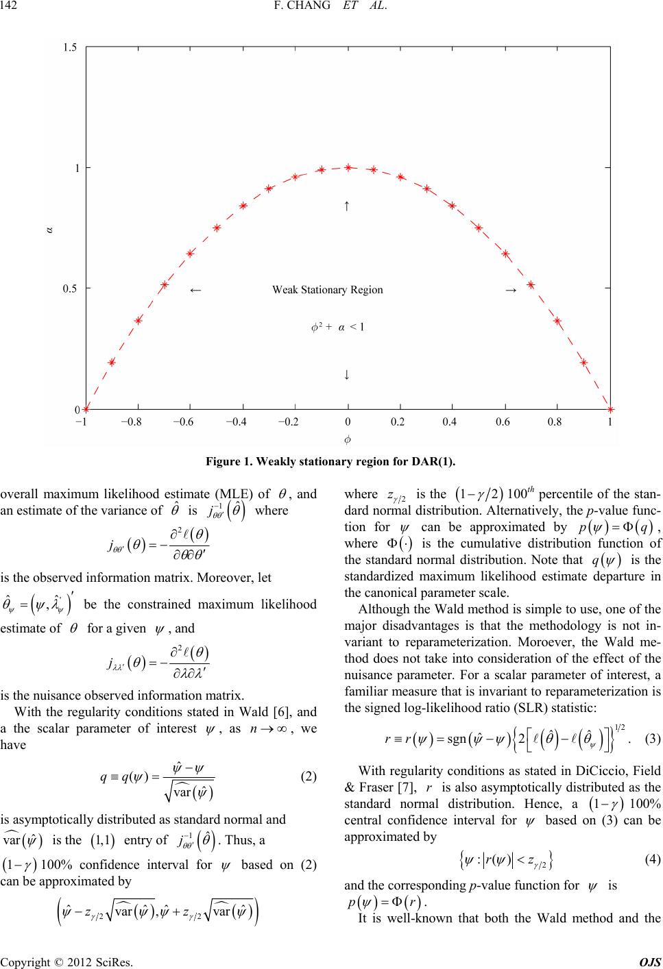

F. CHANG ET AL.
142
Figure 1. Weakly stationary region for DAR(1).
overall maximum likelihood estimate (MLE) of

, and
an estimate of the variance of ˆ

is


1ˆ
j



 
where
2
j







 



is the on matrix. M observed informatioreover, let

'
ˆˆ
,


  be the constrained maximum likel
ihood
estimate of

for a given

, and
 
2
j







 



is the information mtrix.
With the regularity conditions stated in Wald [6], and
nuisance observeda
a the scalar parameter of interest

, as n, we
ha


ve
ˆ
()qq ˆ
var





 (2)
d as standar


ˆ
var
is asymptotically distributed normal and

is the of


1,1 entry

1ˆ
j


. Thus, a


1

1for 00% conce intervnfideal

based
pproxim by on (2) can be aated



where 2 z

is the


 100th percentile of the stan-
dard normal distribution. Alternatively, the p-value func-
tion for
12
can be approximated by




pq   ,
where



 is the cumulative distribution function of
the standard normal distribution. Note that


q

is the
um likel
se, one of th
e Wa
ar parameter of interest, a
fa
standardized maximihood estimate departure in
the canonical parameter scale.
Although the Wald method is simple to ue
major disadvantages is that the methodology is not in-
variant to reparameterization. Moroever, thld me-
thod does not take into consideration of the effect of the
nuisance parameter. For a scal
miliar measure that is invariant to reparameterization is
the signed log-likelihood ratio (SLR) statistic:
 
 

12
ˆˆ
ˆ sgn 2 rr



 

 . (3)
With regularity conditions as stated in DiCiccio, Field
& Fraser [7], r is also asymptotically distributed as the
standard normal distribution. Hence, a

1


100%
central confidence interval for


2
ˆˆˆˆ
varz
 2
, varz




based on (3)
approximated by can be


2
:()rz

  (4)
and the corresponding p-value function for

is




pr   .
It is well-known that both the Wald method and the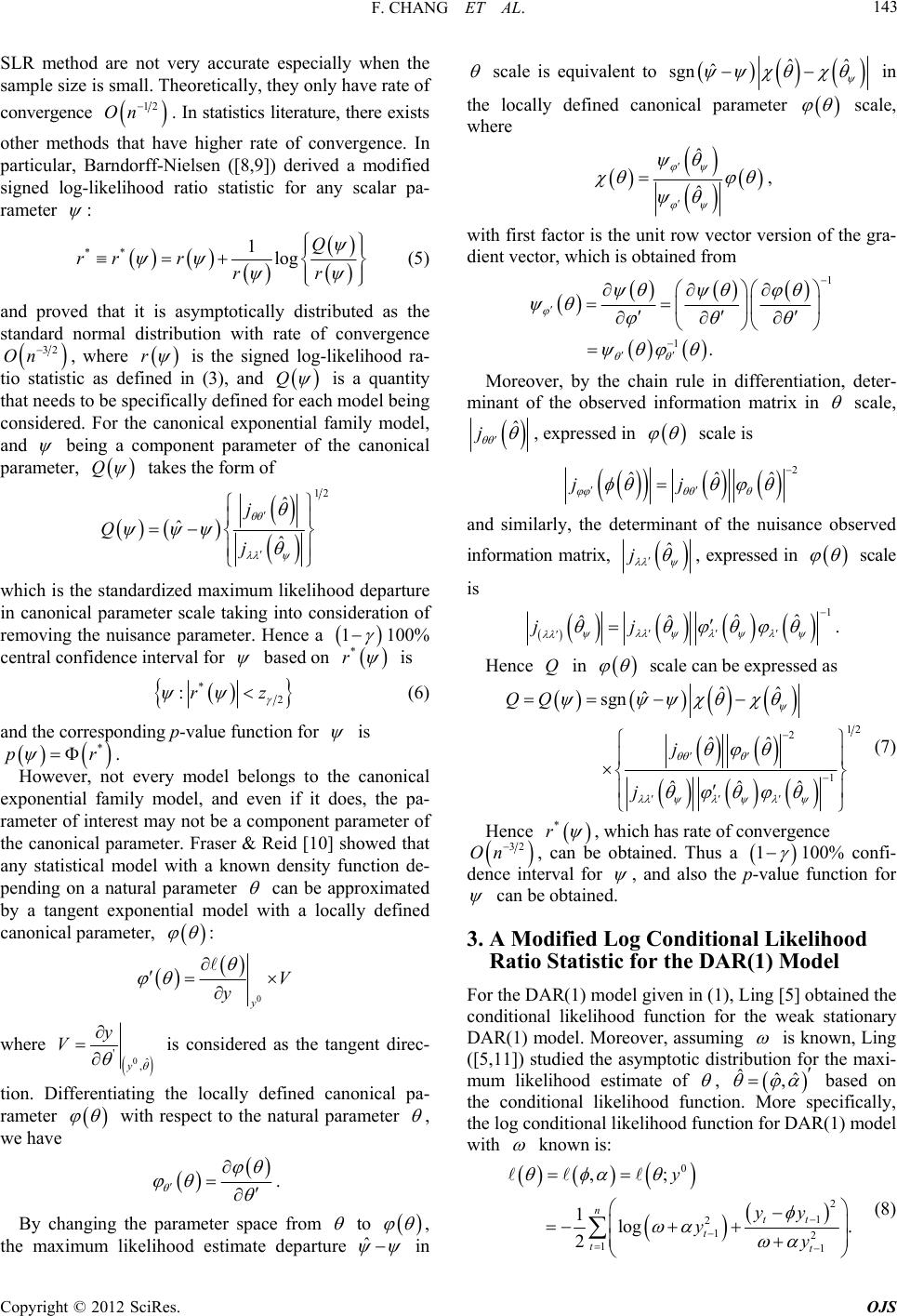

F. CHANG ET AL. 143
SLR method are not very accurate e
sample size is small. Theoretically, they only have rate of
e
specially when the
con ncverge

12
n
. In statistics literaturthere eOe, xis ts
other methods that have higher rate of convergence. In
particular, Barndorff-Nielsen ([8,9]) derived a modified
signed log-likelihood ratio statistic for any scalar pa-
rameter

:
 


** 1log Q
rrrrr

 


 


(5)
and provd that it is asymptotically distributed as the
standard nrm
e
oal distribution with rate of convergence

32,On where

r

is the signed log-likeli
tio statistic as defined i(3), and

Q
hood ra-
n

is a
that needs to d for each model being
quantity
be specifically define
considered. For the canonical exponential family model,
and

bein
ete g a component parameter of the canonical r,

Q
param

takes the form of
 


12
ˆ
ˆˆ
j
Q
j

 

 












which is thdized maximum likelihe standarood departure
in canonical parameter scale taking into consideration of
removing the nuisance parama eter. Hence


1

100%
central confidenrval for ce inte

based on


*
r

is



*2
:rz

  (6)
and the corresponding p-value function for

is


*
pr   .
However, not every model longs to thonical bee can
exponential family model, and even
rameter of interest may not be a component parameter of
al par that
any statistical own density function de-
pe
if it does, the pa-
the canonicameter. Fraser & Reid [10] showed
model with a kn
nding on a natural parameter

can be approximated
by a tangent exponential model with a locally defined
canonical parameter,



 :



0
y
V
y






where

0ˆ
,y
'
y
V

 is considered as the tangent direc-
tion. Differentiating the locally defind canonical pa-
rameter


e




with respect to the eter natural param

,
e

we hav








By chg the parameter space from

.
angin

to



 ,
the maximum likelihood estimure ˆ ate depart



in

scale is equivalent to




ˆˆ
ˆ
sgn


  in
the locally


defined canonical parameter

 scale,
where





ˆ
ˆ



  
,
factor is the unit row vector version of the gra-
dient vector, which is obtained from
 


with first
 
1

 
 

 
1
.





 


 
Moreover, by the chain rule in differentiation, deter-
minant of the observed information matrix in






scale,


ˆ
j




, expressed in
 scale is




  
2
ˆˆˆ
jj
 
  



and simminanisance observed
information matrix,
ilarly, the detert of the nu


ˆ
j
 



, expressed in

 scale
is




 
1
ˆˆ
ˆˆ
jj
  




.
Hence Q in



 scale d as
 
 
can be expresse
 
 
12
2
ˆˆ
ˆ
sgn
ˆˆ
ˆˆˆ
QQ
j
j

   





 
1
 













(7)
Hence


*
r, which has rate of convergence



32
On
, can be obtained. Thus a

1

100% c
dence interval for onfi- , and also the p-value function for


can be obtained.
3. A Modified Log Conditional Likelihood
Fol given in (1), Ling [5] obtained the
conditional likelihood function for the weak stationary
Ratio Statistic for the DAR(1) Model
r the DAR(1) mode
DAR(1) model. Moreover, assuming

is known, Li
([5,11]) studied the asymptotic distribution for the ma ng xi-
mum likelihood estimate of

, ,

ˆˆˆ



 based on
the conditional likelihood function. More specifically,
the log conditional likelihood function for DAR(1) model
with

known is:
 




0
2
1 212
1
,;
1
log.
2
ntt
t
t
y
yy
yy


 







 




 
(8)
1 t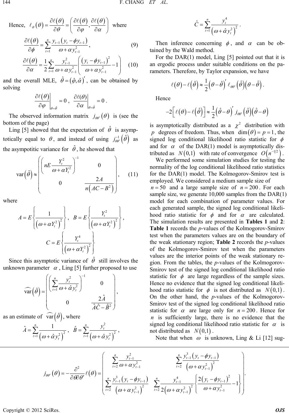

F. CHANG ET AL.
144
Hence,
   
,




 




where 







11
21
ttt
t
yy y
y





, (9)
1
n
t








2
1

 (1
21
122
111
1
2
ntt
t
ttt
yy
y
yy


 










0)
and the

ˆˆˆ
, overall MLE,



,
solving can be obtained by


ˆ
0






, 
ˆ
() 0






.
atriThe observed informax

tion m

j


 is (see the
bottom of the page)
Ling [5] showed that the epectation of ˆ x

is asymp-
totically equal to

, and instnead of usig


1ˆ
j


 as
the asympotitic variance for ˆ

, he showeat d th


1
2


, (
where
20
t
Y
nE 


2
0nA
C B



ˆ
var2
t
Y
A





11)



2
2
1
t
Y




 

, AE

2
2
2
t
t
Y
Y




 

, BE

4
2
2
t
t
Y
CE
Y







Since this asymptotic variance of ˆ

still involves the
unknarameter own p

, Ling [5] further proposed to use


1
2
2
1
2
varˆ
2
0ˆˆˆ
A
0
ˆ
ˆ
n
t
tt
y
y
A
CB




 
,







 


te of


as an estima

ˆ
var

, where

2
2
1
1
ˆn
t
A

ˆt
y

,

2
2
2
1
ˆˆ
n
t
tt
y
B
y



,

4
2
2
1
ˆˆ
n
t
tt
y
C
y



.
Then inference concerning


, and can be ob-
tained by the Wald method.
) model pointed out that it is
s undeconditions on the pa-
rameters. Therefore, by Tayr expansion, we ha


For the DAR(1, Ling [5]
an ergodic procesr suitable
lo ve

1
ˆˆ
ˆˆ
2

 




 .
Hence

 
ˆˆ ˆˆ
22j


1

 





 


is asymptotically distributed as a 2

distribution with
p degrees of freedom. Thus, when

dim 1p 

, the
signed log conditional likelihood ratio statistic for

and for

of the DAR(1) model is asymptotically dis-
tributed as



0,1N with rate of convergence

12.
We performed some simulation studies for testing the
no the log conditional likelihood ratio statistics
for thodel. The Kolmogorov-Smirov test is
employed. We considered a medium sample size of
50n
On
rmality of
e DAR(1) m
and a large sample size of 200n. For each
ple
ameter values.
o

sample size, we generate 10,000 sams from the D AR (1 )
model for each combination of par For
each generated sample, the signed log conditional likeli-
hood rati statistic for

and for

are calculated.
The simulatults are presented in Tables :
Ta ion res 1 and 2
aluesea sta
ble 1 records the p-values of the Kolmogorov-Smirov
test when the parameters values are on the boundary of
the weak stationary region; Table 2 records the p-values
of the Kolmogorov-Smirov test when the parameters
v are the interior points of the wktionary re-
gion. From the tables, the p-values of the Kolmogorov-
Smirov test of the signed log conditional likelihood ratio
statistic for

are large regardless of the sample sizes.
Hence no evidence that th signed log onditional likeli-
hood ratio statistic for e c

is not distributed as


0,1N.
On the other hand, the p-values of the Kolmogorov-
Smirov test of the signed log conditional likelihood ratio
statistic for

are large only for 200n. Hence for
n is sufficiently large, there is no evidence that the
signed log conditional likelihood ratio statistic for

is
not distri buted as


0,1N.
Note that when

is unknown, Ling & Li [12] sug-
 






3
211
122
2
22
1
21
2
34
11 1
1
222
22
22 1
11
.
21
2
nn
ttt
t
tt
tt
nn
tt tt t
t
tt t
tt
yy y
y
yy
yy yy y
y
y
yy

 

 

 




 

 








 


j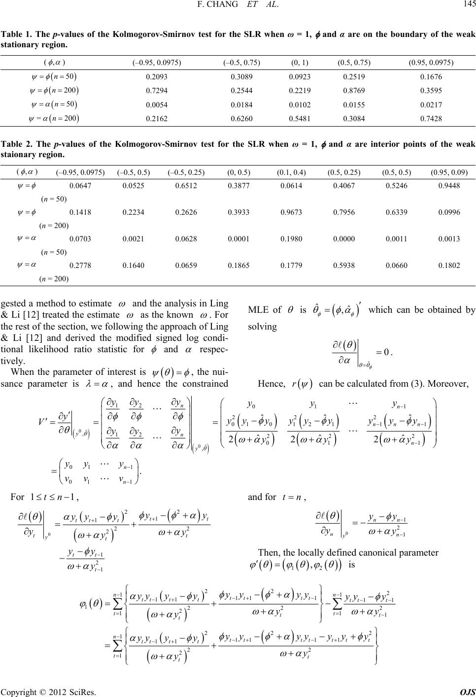






















F. CHANG ET AL.
OJS
145
pe SL Table 1. The -values of the Kolmogorov-Smirnov test for thR when ω = 1,  and α are on the boundary of the weak
stationary region.
(,

 ) (–0.95, 0.0975) (–0..755, 0) (0, 1) (0.5, 0.75) (0.95, 0.0975)

50n   0.2093 0.3089 0.0923 0.2519 0.1676

200n   0.7294 0.2544 0.2219 0.8769 0.3595

0.2162 0.6260 0.5481 0.3084 0.7428

50n   0.0054 0.0184 0.0102 0.0155 0.0217

=200n  
Table 2. The p-values of the Kolmogirnov test for the SLR when,  andinterior points of the weak
staionary region.
(,
orov-Sm ω = 1 α are

 ) (–0.95,.0975) (–0.5, 0.5, 0.25) ((0.1(0.5(0.5, 0.5) , 0.09) 05) (–0.0, 0.5) , 0.4) , 0.25) (0.95
  0.0647 0.0525 0.6512 0.4067 0.5246

0.3877 0614 0.0.9448
(n = 50)

  0.1418 0.2234 0.2626 0.3933 0.9673 0.7956 0.6339 0.0996
(n = 200)

 
n = 50)
0.0703 0.0021 0.0628 0.0001 0.1980 0.0000 0.0011 0.0013
(

 2778 0.1640 0.0659 0.1865 0.1779 0.5938 0.0660 0.1802
n = 200)
0.
(
gested a method ate to estim

and the ann Ling
& Li [12] tate alysis i reated the estim

as the known

. For
the rest ofon, we followine approach of Ling
& Li [12] an the msigncondi
tional likratio statistic for
the secti
d dg th erivedodifieded log -
elihood

and

respec-
vely. er ti When the parameter of intest is


 , the nui-
sance parameter is

 , anhence the consained d tr
LE oMf

is ˆ


ˆ
,


  whibe obby
solving
ch can tained


ˆ
0







.
Hence,


r

can be calculated from (3). Moreover,








0
0
ˆ
,12
ˆ
,2
y
y


 


  
12
22
01
n
y yy
yy
V
 
 





 


 
01 1
2
01 2111
22 2
01 1
01 1
ˆˆ ˆ
ˆˆ ˆ
2 2
.
n
nn n
n
n
n
y
y yyyyyy
y yy yy y
yy y
vv v
 
 







  

  

  








For 11tn ,
yy
y
01 1n
 


0
1
1
22
2
1
21
tt
tt t
tt
yt
tt
t
yy
yyy
yy
y
yy
y
 








 




22
 

and for tn,



0
1
21
nn
nn
y
y
y
y
y








Then, the locally defined canonical parameter






 
12
,






 is








22 2
1 1
11 1
11 11
122 2
2
1
222
1111 1
11
22
2
1
n n
tt tt
tt tttt t
tt
ntttttt
tt tt
tt
t
yy yy
yy yyyy y
yy
y
yyyyy
yy yy
y
y

 
  





 
 
 








 






 





 



11
t
tt
t
y y 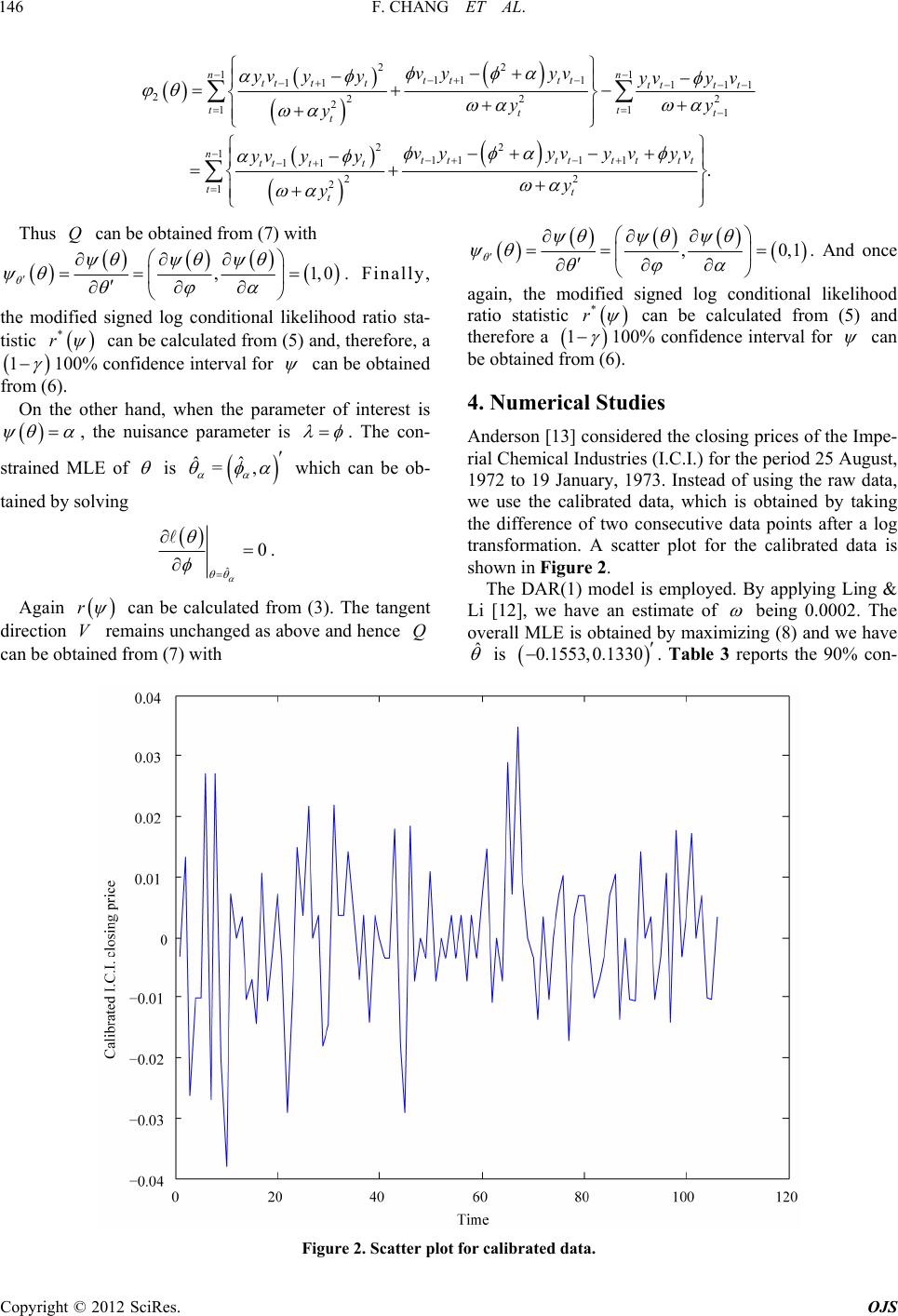



F. CHANG ET AL.
146







22
1 1
11 1
11
222
2
1 1
22
1111 1
11
22
2
1
n n
tt tt
tt tt
t t
t
nttttt t
tt tt
tt
t
vy yv
yv yyyv
y
vyyvy v
yv yy
y
y


 





 
 
 11
1
2
1
.
tt t t
tt
tt
y v
yy
yv















Thus Q can be obtained from (7) with
 
  











 










   
,1,0







. Finally,
nal likelihood ratio sta-
tistic

*
r

 
 





the modified signed log conditio

can be calculated from (5) and, therefore, a
1


100% confidenterval for ce in

can be obtained
om f interest is

fr (6).
On theother hand, when the parameter o

 , the nuisance pter is arame

 
strained MLE
. The con-
of

is

=,
ˆˆ



 which can be ob-
y tainedng

bsolvi
ˆ






r
0 .
Again
 

can be calculated fromhe tangent (3). T
inhanged as a
om (7) wit h
 
,0,1

 
 


 




. And once
again, the modified signed log connal likelihood
ratio statistic
direction V remas uncbove and hence Q
can be obtai ned fr
ditio


*
r

can be calculated from (5) and
therefore a


1100% confidence interval for



can
be obtaine d from (6).
4. Numerical Studies
Anderson [13] considered the closing prices of the Impe-
ary, 1
calibra t
secutive data points after a log
transformation. A scatter plot for the calibrated data is
rial Chemical Industries (I.C.I.) for the period 25 August,
1972 to 19 Janu973. Instead of using the raw data,
we use the ted data, which is obtained byaking
the difference of two con
shown in Figure 2.
The DAR(1) model is employed. By applying Ling &
Li [12], we have an estimate of

being 0.0002. The
overall MLE is obtained by maximizing (8) and we have
ˆ

is

0.1553,0.1330

. Table 3 reports the 90% con-
Figure 2. Scatter plot for calibrated data.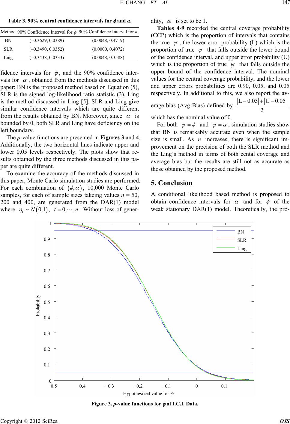

F. CHANG ET AL. 147
Table 3. 90% central confidence intervals for
 and α.
Method 90% Confidence Interval for  90% Confidence Interval for α

BN (–0.3629, 0.03 89 ) (0.0048, 0.4719)
SLR (–0.3490, 0.0352) (0.0 0 00 , 0.4072)
Ling (–0.3438, 0.0333) (0.0048, 0.3588)
fidervals for nce inte

, and the 90% confidence inter-
vals for

, obtained from the methods discussed in this
paper: is the proposed method based on Equatio n (5),
SLR is te signed log-likelihood ratio statistic (3), Ling
is the mhod discussed in Ling [5]. SLR and Ling give
similar confidence intervals which are quite different
from thlts obtained by BN. Moreover, since
BN
h
et
e resu

is
bounded by 0, both SLR and Ling have deficiency on the
left boundary.
The p-value functions are presented in Figures 3 and 4.
Additionally, the two horizontal lines indicate upper and
lower 0.05 levels respectively. The plots show that re-
sults obtained by the three methods discussed in this pa-
per are quite different.
To examine the accuracy of the methods discussed in
this paper, Monte Carlo simulation studies are performed.
For each coon of

, mbinati

 , 10,000 Monte Carlo
samples, for each sample sizes takeing values n = 50,
200 and 4 are generated from the DAR(1) model
, 0,,tn. Withou
ality,
of
00,

0, 1N where t  
is set to be 1.
Tables 4-9 recorded the central coverage probability
(CCP) which is the proportion of intervals that contains
the true

, the lower error probability (L) which is the
proportion of true

that falls outside the lower bound
of the confidence interval, and upper error probability (U)
which is the proportion of true

that falls outside the
upper bound of the confidence interval. The nominal
values for the central coverage pro bability, and the lower
and upper errors probabilities are 0.90, 0.05, and 0.05
respectively. In additional to this, we also report the av-
erage bias (Avg Bias) defined by L0.05U 0.05
2
,
which has the nominal value of 0.
For both
t loss of gener-

 and




, simulation studies show
that BN is remarkably accurate even when the sample
size is small. As n increases, there is significant im-
provement on the precision of both the SLR method and
the Ling’s method in terms of both cental coverage and
average bias but the results are still not as accurate as
those obtained by the proposed method.
5. Conclusion
A conditional likelihood based method is proposed to
obtain confidence intervals for and for


of the
weak stationary DAR(1) model. Theoretically, the pro-
Figure 3. p-value functions for  of I.C.I. Data.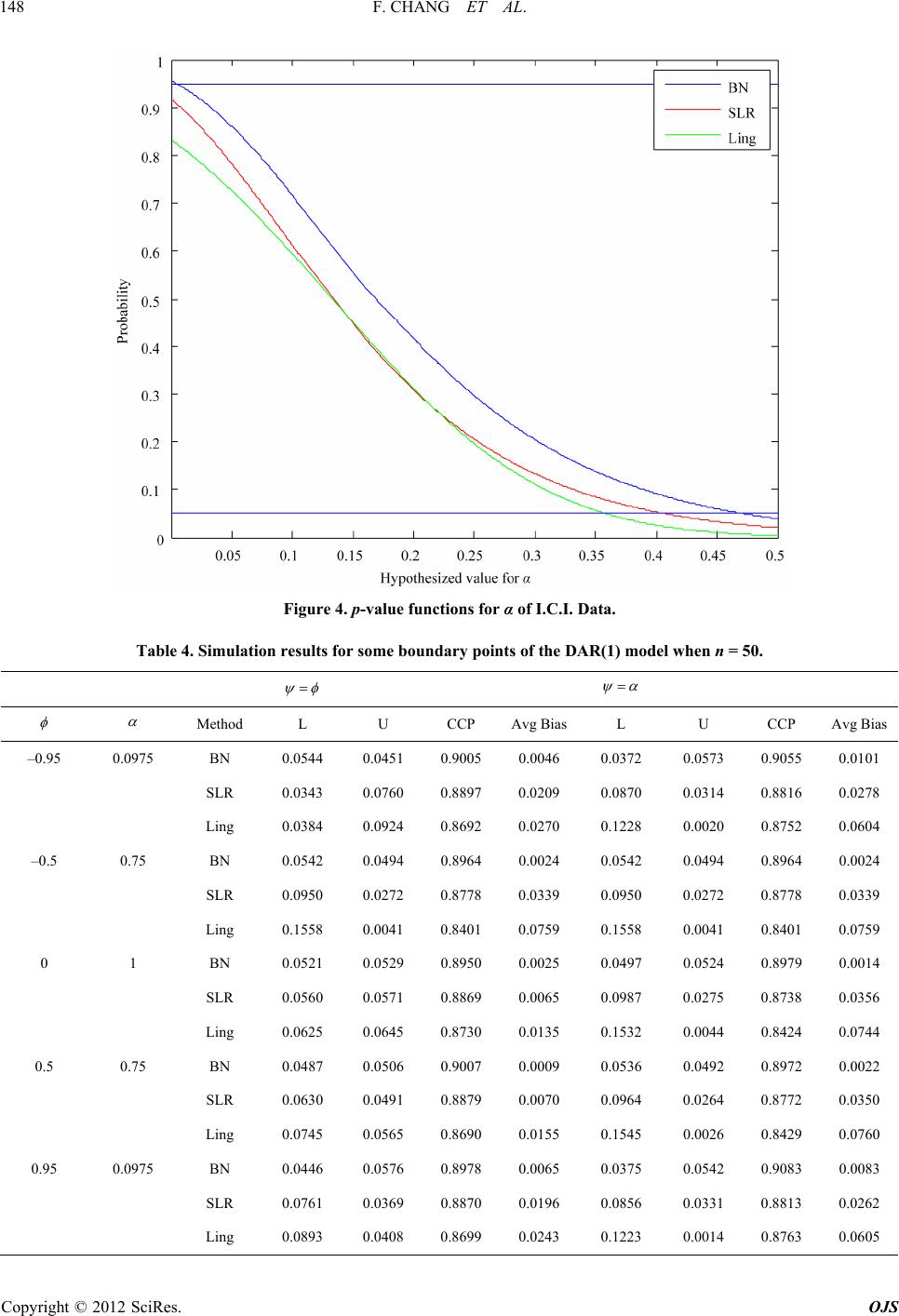

F. CHANG ET AL.
148
Figure 4. p-value functions for α of I.C.I. Data.
Table 4. Simulation results for some boundary points of the DAR(1) model when n = 50.

 




Me th od L U CCP Avg BiasL U CCP A vg Bias

–0.95 0.0975 BN 0.0544 0.0451 0.9005 0.0046 0.0372 0.0573 0.9055 0.0101
SLR 0.0343 0.0760 0.8897 0.0209 0.0870 0.0314 0.8816 0.0278
Ling 0.0384 0.0924 0.8692 0.0270 0.1228 0.0020 0.8752 0.0604
–0.5 0.75 BN 0.0542 0.0494 0.8964 0.0024 0.0542 0.0494 0.8964 0.0024
SLR 0.0950 0.0272 0.8778 0.0339 0.0950 0.0272 0.8778 0.0339
Ling 0.1558 0.0041 0.8401 0.0759 0.1558 0.0041 0.8401 0.0759
0 1 BN 97 0.0524 0.8979 0.0014
SLR 0.0560 0.0571 0.8869 0.0065 0.0987 0.0275 0.8738 0.0356
Ling 0.0625 0.0645 0.8730 0.0135 0.1532 0.0044 0.8424 0.0744
0.5 0.75 BN 0.0487 0.0506 0.9007 0.0009 0.0536 0.0492 0.8972 0.0022
SLR 0.0630 0.0491 0.8879 0.0070 0.0964 0.0264 0.8772 0.0350
Ling 0.0745 0.0565 0.8690 0.0155 0.1545 0.0026 0.8429 0.0760
0.95 0.0975 BN 0.0446 0.0576 0.8978 0.0065 0.0375 0.0542 0.9083 0.0083
SLR 0.0761 0.0369 0.8870 0.0196 0.0856 0.0331 0.8813 0.0262
Ling 0.0893 0.0408 0.8699 0.0243 0.1223 0.0014 0.8763 0.0605
0.0521 0.0529 0.8950 0.0025 0.04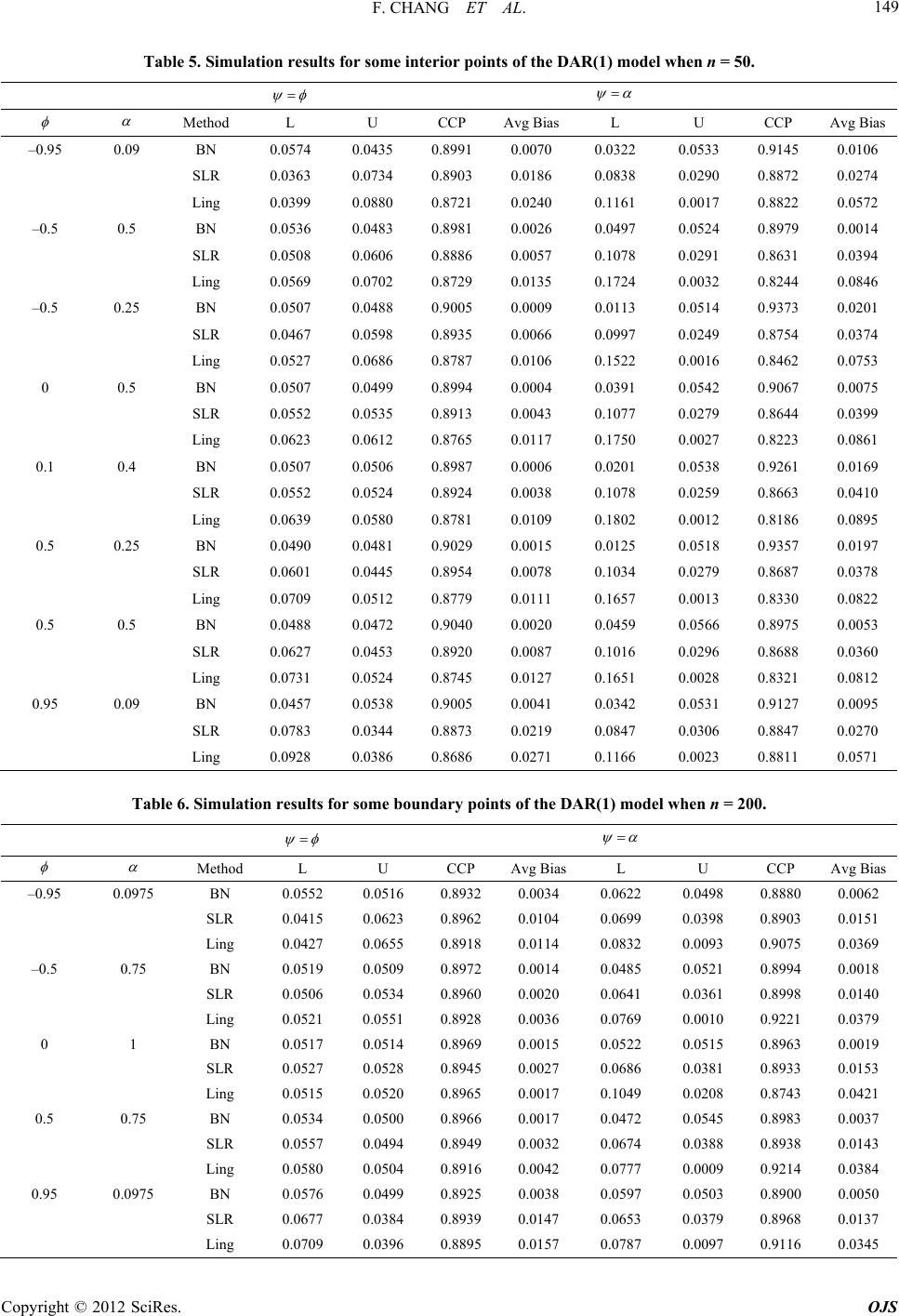

F. CHANG ET AL. 149
Table 5. Simulation results for some interior points of the DAR(1) model when n = 50.

 




Method L U CCP Avg BiasL U CCP Avg Bias

–0.95 0.09 BN 0.0574 0.0435 0.8991 0.0070 0.0322 0.0533 0.9145 0.0106
SLR 0.0363 0.0734 0.8903 0.0186 0.0838 0.0290 0.8872 0.0274
Ling 0.0399 0.0880 0.8721 0.0240 0.1161 0.0017 0.8822 0.0572
–0.5 0.5 BN 0.0536 0.0483 0.8981 0.0026 0.0497 0.0524 0.8979 0.0014
SLR 0.0508 0.0606 0.8886 0.0057 0.1078 0.0291 0.8631 0.0394
Ling 0.0569 0.0702 0.8729 0.0135 0.1724 0.0032 0.8244 0.0846
–0.5 0.25 BN 0.0507 0.0488 0.9005 0.0009 0.0113 0.0514 0.9373 0.0201
SLR 0.0467 0.0598 0.8935 0.0066 0.0997 0.0249 0.8754 0.0374
Ling 0.0527 0.0686 0.8787 0.0106 0.1522 0.0016 0.8462 0.0753
0 0.5 BN 0.0507 0.0499 0.8994 0.0004 0.0391 0.0542 0.9067 0.0075
SLR 0.0552 0.0535 0.8913 0.0043 0.1077 0.0279 0.8644 0.0399
Ling 0.0623 0.0612 0.8765 0.0117 0.1750 0.0027 0.8223 0.0861
0.1 0.4 BN 0.0507 0.0506 0.8987 0.0006 0.0201 0.0538 0.9261 0.0169
SLR 0.0552 0.0524 0.8924 0.0038 0.1078 0.0259 0.8663 0.0410
Ling 0.0639 0.0580 0.8781 0.0109 0.1802 0.0012 0.8186 0.0895
0.5 0.25 BN 0.0490 0.0481 0.9029 0.0015 0.0125 0.0518 0.9357 0.0197
SLR 0.0601 0.0445 0.8954 0.0078 0.1034 0.0279 0.8687 0.0378
Ling 0.7 0.0013 0.8330 0.0822
0.5 0.5 BN 0.0488 0.0472 0.9040 0.0020 0.0459 0.0566 0.8975 0.0053
88 0.0360
Ling 0.0731 0.0524 0.8745 0.0127 0.1651 0.0028 0.8321 0.0812
0.95 0.09 BN 0.0457 0.0538 0.9005 0.0041 0.0342 0.0531 0.9127 0.0095
0.0783 0.0344 0.0.0847 0.0306 0.
Li 0.0.00
0709 0.0512 0.8779 0.0111 0.165
SLR 0.0627 0.0453 0.8920 0.0087 0.1016 0.0296 0.86
SLR 8873 0.0219 8847 0.0270
ng 0928 0386 .8686 .0271 0.1166 0.0023 0.8811 0.0571
Table 6. Simulation ror sundnts AR(1) model w 20esults fome boary poiof the Dhen n =0.

 





M AAethodL U CCP vg BiasL U CCP vg Bias
–0.0.0975 95 BN 0.0552 0.0516 0.8932 0.0034 0.0622 0.0498 0.8880 0.0062
SLR
Ling
0.0415
0.0427
0.0623
0.0655
0.8962
0.8918
0.0104
0.0114 0.
0.0699
0832 0.
0.0398
0093
0.8903
0.9075
0.0151
0.0369
–0.
0 1
0.5 0.75 BN 0.0534 0.0500 0.8966 0.0017 0.0472 0.0545 0.8983 0.0037
0. 0.0975
SLR 0.0677 0.0384 0.8939 0.0147 0.0653 0.0379 0.8968 0.0137
0.5 75BN 0.0519 0.0509 0.8972 0.0014 0.0485 0.0521 0.8994 0.0018
SLR 0.0506 0.0534 0.8960 0.0020 0.0641 0.0361 0.8998 0.0140
Ling
BN
0.0521
0.0517
0.0551
0.0514
0.8928
0.8969
0.0036 0.
0.0015 0.
0769 0.
0522 0.
0010
0515
0.9221
0.8963
0.0379
0.0019
SLR 0.0527 0.0528 0.8945 0.0027 0.0686 0.0381 0.8933 0.0153
Ling 0.0515 0.0520 0.8965 0.0017 0.1049 0.0208 0.8743 0.0421
SLR 0.0557 0.0494 0.8949 0.0032 0.0674 0.0388 0.8938 0.0143
Ling 0.0580 0.0504 0.8916 0.0042 0.0777 0.0009 0.9214 0.0384
95BN 0.0576 0.0499 0.8925 0.0038 0.0597 0.0503 0.8900 0.0050
Ling 0.0709 0.0396 0.8895 0.0157 0.0787 0.0097 0.9116 0.0345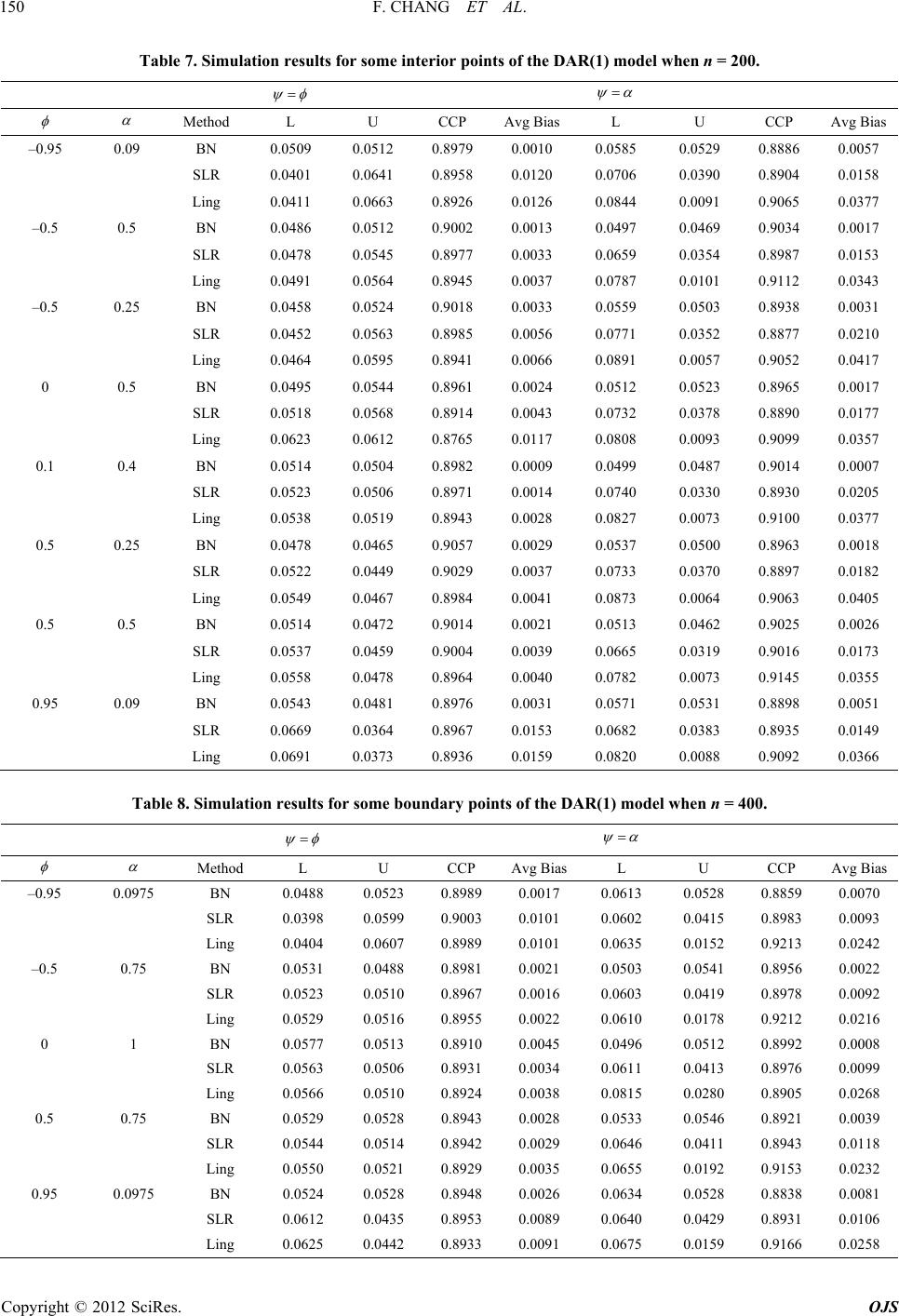

F. CHANG ET AL.
150
Table 7. Simulation results for some interior points of the DAR(1) model when n = 200.

 





Method L U CCP Avg BiasL U CCP Avg Bias
–0.95 0.09 BN 0.0509 0.0512 0.8979 0.0010 0.0585 0.0529 0.8886 0.0057
SLR 0.0401 0.0641 0.8958 0.0120 0.0706 0.0390 0.8904 0.0158
Ling 0.0411 0.0663 0.8926 0.0126 0.0844 0.0091 0.9065 0.0377
–0.5 0.5 BN 0.0486 0.0512 0.9002 0.0013 0.0497 0.0469 0.9034 0.0017
SLR 0.0478 0.0545 0.8977 0.0033 0.0659 0.0354 0.8987 0.0153
Ling 0.0491 0.0564 0.8945 0.0037 0.0787 0.0101 0.9112 0.0343
–0.5 0.25 BN 0.0458 0.0524 0.9018 0.0033 0.0559 0.0503 0.8938 0.0031
SLR 0.0452 0.0563 0.8985 0.0056 0.0771 0.0352 0.8877 0.0210
Ling 0.0464 0.0595 0.8941 0.0066 0.0891 0.0057 0.9052 0.0417
0 0.5 BN 0.0495 0.0544 0.8961 0.0024 0.0512 0.0523 0.8965 0.0017
SLR 0.0518 0.0568 0.8914 0.0043 0.0732 0.0378 0.8890 0.0177
Ling 0.0623 0.0612 0.8765 0.0117 0.0808 0.0093 0.9099 0.0357
0.1 0.4 BN 0.0514 0.0504 0.8982 0.0009 0.0499 0.0487 0.9014 0.0007
SLR 0.0523 0.0506 0.8971 0.0014 0.0740 0.0330 0.8930 0.0205
Ling 0.0538 0.0519 0.8943 0.0028 0.0827 0.0073 0.9100 0.0377
0.5 0.25 BN 0.0478 0.0465 0.9057 0.0029 0.0537 0.0500 0.8963 0.0018
SLR 0.0522 0.0449 0.9029 0.0037 0.0733 0.0370 0.8897 0.0182
Ling 0.0549 0.0467 0.8984 0.0041 0.0873 0.0064 0.9063 0.0405
0.5 0.5 BN 0.0514 0.0472 0.9014 0.0021 0.0513 0.0462 0.9025 0.0026
SLR 0.0537 0.0459 0.9004 0.0039 0.0665 0.0319 0.9016 0.0173
Ling 0.0558 0.0478 0.8964 0.0040 0.0782 0.0073 0.9145 0.0355
0.95 0.09 BN 0.0543 0.0481 0.8976 0.0031 0.0571 0.0531 0.8898 0.0051
SLR 0.0669 0.0364 0.8967 0.0153 0.0682 0.0383 0.8935 0.0149
Ling 0.0691 0.0373 0.8936 0.0159 0.0820 0.0088 0.9092 0.0366
Table 8. Simulation results for some boundary points of the DAR(1) model when n = 400.

 





Me th od L U CCP Avg BiasL U CCP Avg Bias
–0.95 0.0975 BN 0.0488 0.0523 0.8989 0.0017 0.0613 0.0528 0.8859 0.0070
SLR 0.0398 0.0599 0.9003 0.0101 0.0602 0.0415 0.8983 0.0093
Ling 0.0404 0.0607 0.8989 0.0101 0.0635 0.0152 0.9213 0.0242
–0.5 0.75 BN 0.0531 0.0488 0.8981 0.0021 0.0503 0.0541 0.8956 0.0022
SLR 0.0523 0.0510 0.8967 0.0016 0.0603 0.0419 0.8978 0.0092
Ling 0.0529 0.0516 0.8955 0.0022 0.0610 0.0178 0.9212 0.0216
0 1 BN 0.0577 0.0513 0.8910 0.0045 0.0496 0.0512 0.8992 0.0008
SLR 0.0563 0.0506 0.8931 0.0034 0.0611 0.0413 0.8976 0.0099
Ling 0.0566 0.0510 0.8924 0.0038 0.0815 0.0280 0.8905 0.0268
0.5 0.75 BN 0.0529 0.0528 0.8943 0.0028 0.0533 0.0546 0.8921 0.0039
SLR 0.0544 0.0514 0.8942 0.0029 0.0646 0.0411 0.8943 0.0118
Ling 0.0550 0.0521 0.8929 0.0035 0.0655 0.0192 0.9153 0.0232
0.95 0.0975 BN 0.0524 0.0528 0.8948 0.0026 0.0634 0.0528 0.8838 0.0081
SLR 0.0612 0.0435 0.8953 0.0089 0.0640 0.0429 0.8931 0.0106
Ling 0.0625 0.0442 0.8933 0.0091 0.0675 0.0159 0.9166 0.0258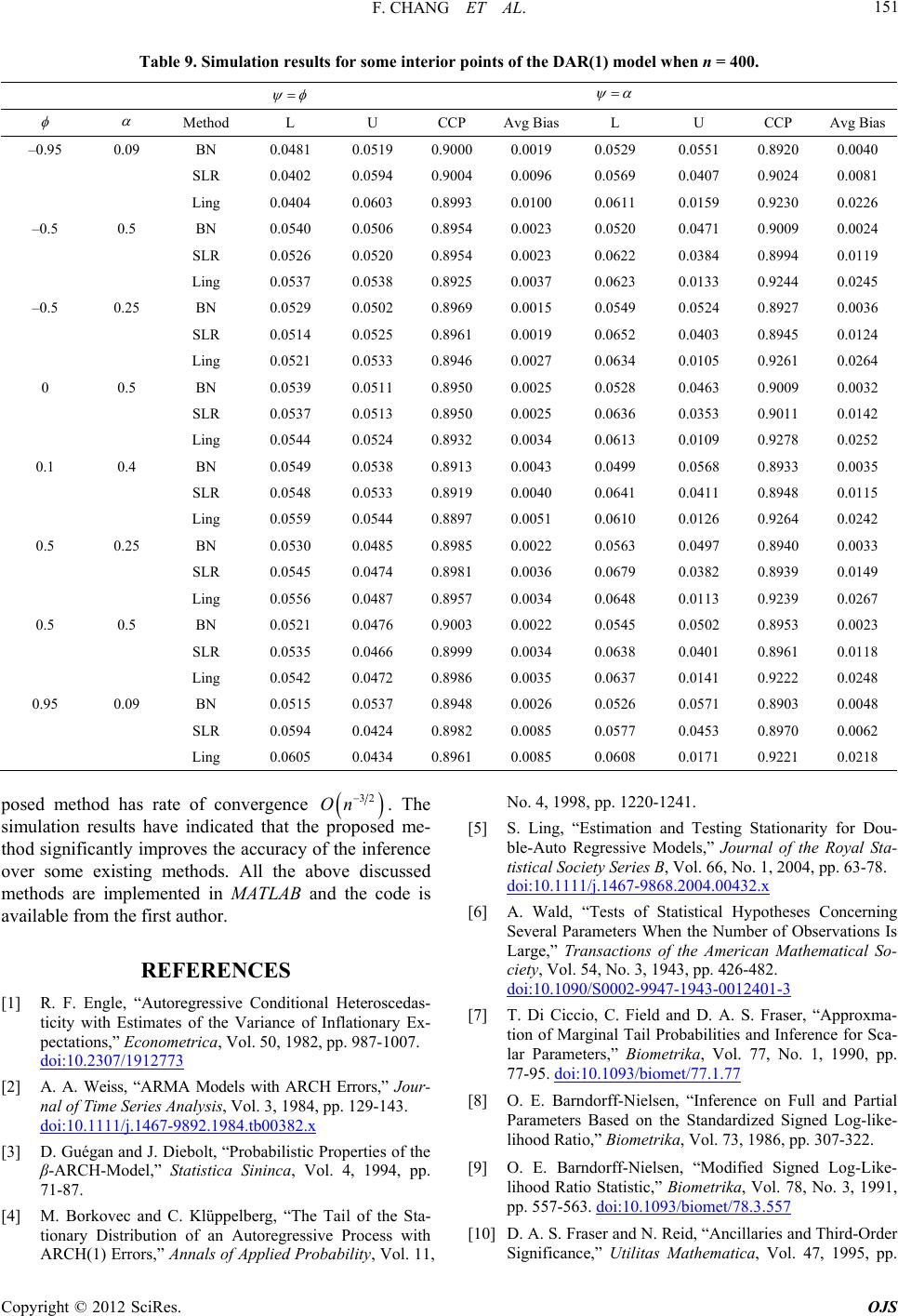

F. CHANG ET AL.
151
Table 9. Simulation results for some interior points of the DAR(1) model when n = 400.

 





Method L U CCP Avg BiasL U CCP Avg Bias
–0.95 0.09 BN 0.0481 0.0519 0.9000 0.0019 0.0529 0.0551 0.8920 0.0040
SLR 0.0402 0.0594 0.9004 0.0096 0.0569 0.0407 0.9024 0.0081
Ling 0.0404 0.0603 0.8993 0.0100 0.0611 0.0159 0.9230 0.0226
–0.5 0.5 BN 0.0540 0.0506 0.8954 0.0023 0.0520 0.0471 0.9009 0.0024
SLR 0.0526 0.0520 0.8954 0.0023 0.0622 0.0384 0.8994 0.0119
Ling 0.0537 0.0538 0.8925 0.0037 0.0623 0.0133 0.9244 0.0245
–0.5 0.25 BN 0.0529 0.0502 0.8969 0.0015 0.0549 0.0524 0.8927 0.0036
SLR 0.0514 0.0525 0.8961 0.0019 0.0652 0.0403 0.8945 0.0124
Ling 0.0521 0.0533 0.8946 0.0027 0.0634 0.0105 0.9261 0.0264
0 0.5 BN 0.0539 0.0511 0.8950 0.0025 0.0528 0.0463 0.9009 0.0032
SLR 0.0537 0.0513 0.8950 0.0025 0.0636 0.0353 0.9011 0.0142
Ling 0.0544 0.0524 0.8932 0.0034 0.0613 0.0109 0.9278 0.0252
0.1 0.4 BN 0.0549 0.0538 0.8913 0.0043 0.0499 0.0568 0.8933 0.0035
SLR 0.0548 0.0533 0.8919 0.0040 0.0641 0.0411 0.8948 0.0115
Ling 0.0559 0.0544 0.8897 0.0051 0.0610 0.0126 0.9264 0.0242
0.5 0.25 BN 0.0530 0.0485 0.8985 0.0022 0.0563 0.0497 0.8940 0.0033
SLR 0.0545 0.0474 0.8981 0.0036 0.0679 0.0382 0.8939 0.0149
Ling 0.0556 0.0487 0.8957 0.0034 0.0648 0.0113 0.9239 0.0267
0.5 0.5 BN 0.0521 0.0476 0.9003 0.0022 0.0545 0.0502 0.8953 0.0023
SLR 0.0535 0.0466 0.8999 0.0034 0.0638 0.0401 0.8961 0.0118
Ling 0.0542 0.0472 0.8986 0.0035 0.0637 0.0141 0.9222 0.0248
0.95 0.09 BN 0.0515 0.0537 0.8948 0.0026 0.0526 0.0571 0.8903 0.0048
SLR 0.0594 0.0424 0.8982 0.0085 0.0577 0.0453 0.8970 0.0062
Ling 0.0605 0.0434 0.8961 0.0085 0.0608 0.0171 0.9221 0.0218
posed method has rate of convergence

32
On
. The No. 4, 1998, pp. 1220-1241.
simulation results have indat the proposed me-
thod significantly improves the inference
over sme existing methll theove dissed
meented TL this
available from the first auth
EFER CE
[1] . F. Engle,Autoregr ConHetas-
ity with Estimates ofarianflat
ctations,” nometric ol. 50p. 9.
i:10.2307/1912773
icated th
e accuracy of th
oods. A abscu
thods are implemin MA AB ande code
or.
RENS
R “essiveditional erosced
tic the Vce of Inionary Ex-
pe Eco a, V, 1982, p87-1007
do
[2] . A. Weiss,RMA M with Errr-
:10.1111 00
A “Aodels ARCHors,” Jou
nal of Time Series Analysis
/j.1467-9892.1984.tb
, Vol. 3, 1984, pp. 129-143.
doi 382.x
[3] . Guégan and J. Dieboobabope
Stati Sinin. 4, p.
7.
[4] . Borkovecd C. Klüppelberg,ail ota-
nary Distrtion of an Autore Proith
RCH(1) Errs,” Annappliebili
[5] S. Lng, “Estimation and Testing Stationarity for Dou-
ble-Auto Regressive Models,” Journal f the RoyaSta-
ciety Ses B, Vol. 66, No. 14, p
doi:10.1111/j68.432
Dlt, “Prilistic Prrties of the
β-ARCH-Model,” stica ca, Vol1994, p
71-8
M an “The Tf the S
tio
Aibu ro gressive d Proba
cess w
ty, Vol. 11, ls of A
i
ol
tistical Soeri, 200p. 63-78.
.1467-98 2004.00.x
[6] A, “TStaHypotheses Cog
Se ramenrva
Lrica ema-
cl. 546-4
doi:10.1090/S 47- 124
. Waldests of tistical ncernin
veral Pa
arge,” Transactions of
ters Whe the Numbe
the Ame
r of Obse
n Math
tions Is
tical So
iety, Vo, No. 3, 1943, pp. 4282.
0002-99 1943-0001-3
[7] T. Di Cicciod an S.“A-
targ Pros anence for Sca-
lete metr l. 71, 1990, pp.
7i:10ome 7
, C. Field D. A. Fraser, pproxma
ion of M
ar Paraminal Tail rs,” Bio
babilitie
ika, Vod Infer 7, No.
7-95. do.1093/bit/77.1.7
Orndsen,ncel anal
Parameters Based on therdized -
ltio, rika 3, 1
O. E. BarndlsenifieL-
latio Statistic,” B, Vol. 78, No. 3, 1991,
pp. 557-563. doi:10.1093/b
[8] . E. Baorff-Niel “Infere on Fuld Parti
Standaed SignLog-like
ihood Ra” Biomet , Vol. 7986, pp. 307-322.
[9] orff-Nie, “Modd Signed og-Like
ihood Riometrika
iomet/78.3.557
[10] D. Fraser Reid Third-Order
S nce,s Mica7, .
A. S.
ignifica and N. ” Utilita
, “Ancillaries and
athemat, Vol. 41995, pp

F. CHANG ET AL.
152
33-53.
[11] , “Aouble AR) Model: Struture andstima-
Statistica Sinica, Vol. 17, 2007, pp. 161-175.
[12] S. Ling and D. Li, “otic Innce for onsta-
ka, Vol. 95, No. 1,
2008, pp. 257-263. /biomet/asm084
D. Ling
tion,” D(pc E
Asymptferea N
tionary Double AR(1) Model,” Biometri
doi:10.1093
[13] O. D. Anderson, “Time Ser Analysis Forecasting:
-Jenkins Approachutterw976
ies and
The Box,” Borth, 1.