Modification of water application uniformity among closed circuit trickle irrigation systems

doi:10.4236/as.2010.11001

Paper Menu >>

Journal Menu >>

Vol.1, No.1, 1-9 (2010)

doi:10.4236/as.2010.11001

Agricultural Sciences

Modification of water application uniformity among

closed circuit trickle irrigation systems

Hani A.-G. Mansour1*, Mohamed Yousif Tayel1, Mohamed A. Abd El-Hady1,

David A. Lightfoot2, Abdel-Ghany Mohamed El-Gindy3

1Water Relations and Field Irrigation Department, National Research Centre, Giza, Egypt; *Corresponding Author:

hanimansour88@yahoo.com

2Soil & Plant and Agricultural Systems Department, Southern Illinois University, Carbondale, USA

3Agricultural Engineering Department, Faculty of Agriculture, Ain Shams University, Cairo, Egypt

Received 2 April 2010; revised 30 April 2010; accepted 5 May 2010.

ABSTRACT

The aim of this research was determine the ma-

ximum application uniformity of closed circuit

trickle irrigation systems designs. Laboratory

test s carried out for Two ty pes of closed circuit s:

a) One manifold for lateral lines or Closed cir-

cuits with One Manifold of Trikle Irrigation Sys-

tem (COMTIS); b) Closed circuits with Two

Manifolds of Trikle Irrigation System (CTMTIS),

and c) Traditional Trik le Irrigation System (TTIS)

as a control. Three lengths of lateral lines were

used, 40, 60, and 80 meters. PE tubes lateral

lines: 16 mm diameter; 30 cm emitters distance,

and GR built-in emitters 4 lph when operating

pressure 1 bar. Experiments were conducted at

the Agric. Eng. Res. Inst., ARC, MALR, Egypt.

With COMTIS the emitter flow rate was 4.07, 3.51,

and 3.59 lph compared to 4.18, 3.72, and 3.71 lph

with CTMTIS and 3.21, 2.6, and 2.16 lph with TTIS

(lateral lengths 40, 60, and 80 meters respec-

tively). Uniformi ty varied widely within individual

lateral lengths and between circuit types. Under

CTMTIS uniformity values were 97.74, 95.14, and

92.03 %; with COMTIS they were 95.73, 89.45,

and 83.25 %; and with TTIS they were 88.27,

84.73, and 80.53 % (for lateral lengths 40, 60, 80

meters respectively). The greatest uniformity

was observed under CTMTIS and COMTIS w hen

using the shortest lateral length 40 meters, then

lateral length 60 meters, while the lowest value

was observed when using lateral length 80 me-

ters this result depends on the physical and hy-

draulic characteristics of the emitter and lateral

line. CTMTIS was more uniform than either

COMTIS or TTIS. Friction losses w ere decreased

with CTMTIS in the emitter laterals at lengths 40

meters compared to TTIS and COMTIS. There-

fore, differences may be related to increased

friction losses when using TDIS and COMDIS.

Keywords: Trickle Irrigation; Closed Circuits;

Manifold; Lateral; Flow Rate; Uniformity

1. INTRODUCTION

Trickle irrigation has been used since ancient times when

buried clay pots were filled with water, which would

gradually seep into the grass. Perforated pipe was intro-

duced in Germany in the 1920s and in 1934, Nobey ex-

perimented with irrigating through porous canvas hose at

Michigan State University. Plastic microtubing and vari-

ous types of emitters began to be used in the greenhouses

of Europe and the United States.

Qualitative classification standards for the production

of emitters, the emitter discharge rate q (m3/h) has been

described by a power law, =

qkH, where operating

pressure head H (m), emitter coefficient (k), and expo-

nent (x) depend on emitter characteristics [1]. Capra and

Scicolone [2] indicated that the major sources of emitter

flow rate variations are emitter design, the material used

to manufacture the lateral line, and precision. According

to [3] the main factors affecting trickle irrigation system

uniformity are: 1) manufacturing variations in emitters

and pressure regulators, 2) pressure variations caused by

elevation changes, 3) friction head losses throughout the

pipe network, 4) emitter sensitivity to pressure and irriga-

tion water temperature changes, and 5) emitter clogging.

Similarly, according to the manufacturer’s coefficient of

emitter variation (CVm), have been developed by ASAE.

CVm values below 10% are suitable and > 20% are un-

acceptable [4]. The emitter discharge variation rate (qvar)

should be evaluated as a design criterion in trickle irriga-

tion systems; qvar < 10% may be regarded as good and

qvar > 20% as unacceptable [5,6]. The acceptability of

micro-irrigation systems has also been classified accord-

H. A.-G. Mansour et al. / Agricultural Sciences 1 (2010) 1-9

ing to the statistical parameters, Uqs and EU; namely, EU

= 94%-100% and Uqs = 95%-100% are excellent, and

EU < 50% and Uqs < 60% are unacceptable [7]. Ortega

et al [8] calculated emission uniformity (EU), pressure

variation coefficient (VCp), and flow variation coeffi-

cient per emitter (VCq) at localized systems and reported

that they were 84.3%, 0.12, and 0.19, respectively. They

classified the systems unacceptable for VCq > 0.4 and

excellent for VCq < 0.1. In addition to pressure variation

along irrigation tape, variation in emitter structure or

emitter geometry has been known to cause poor uniform-

ity of emitter discharge [1,5,9]. Differences in emitter

geometry may be caused by variation in injection pres-

sure and heat instability during their manufacture, as well

as by a heterogeneous mixture of materials used for the

production [1]. Berkowitz [10] observed reductions in

emitter irrigation flow ranging from 7 to 23% at five sites

observed. Reductions in scouring velocities were also

observed from the designed 0.6 m/s (2ft/s) to 0.3 m/s

(1ft/s). Lines also developed some slime build-up, as

reflected by the reduction in scouring velocities, but this

occurred to a less degree with higher quality effluent. In

their treatments they generally used approximate friction

equations such as Hazen-Williams and Scobey, neglected

the variation of the velocity head along the lateral and

assumed initial uniform emitter flow. Warrick & Yitayew

[11] assumed a lateral with a longitudinal slot and pre-

sented design charts based on spatially varied flow. The

latter solution has neglected the presence of laminar flow

in a considerable length of the downstream part of the

lateral. Hathoot et al [12] provided a solution based on

uniform emitter discharge but took into account the

change of velocity head and the variation of Reynold’s

number. They used the Darcy-Weisbach friction equation

in estimating friction losses. Hathoot et al [13] consid-

ered individual emitters with variable outflow and pre-

sented a step by step computer program for designing

either the diameter or the lateral length. In this study we

considered the pressure head losses due to emitters pro-

trusion. These losses occur when the emitter barb protru-

sion obstructs the water flow. Three sizes of emitter barbs

were specified, small, medium and large in which the

small barb has an area equal or less than 20 mm², the

medium barb has an area between 21-31mm² and the

large one has an area equal to or more than 32 mm². The

objectives of the present research were:

1) Recovery the problem of pressure reduction at the

end stage of lateral lines.

2) Investigate emitter discharge application uniformity

and its dependence on operation pressures and Laterals

lengths (40, 60, and 80 m).

3) To compare emitter discharge uniformity between

tow type of closed circuits (COMTIS and CTMTIS) and

traditional trickle system (TTIS).

2. MATIRIALS AND METHODS

2.1. Site Location and Experimental Design

This experiment was conducted at Irrigation Devices and

Equipments Tests Laboratory, Agricultural Engineering

Research Institute, Agriculture Research Center, Cairo,

Egypt. The experimental design was randomized com-

plete block with three replicates. Three irrigation new

lateral lines 40, 60, 80 m long that were installed at con-

stant level and under ten operating pressures 0.2, 0.4, 0.6,

0.8, 1.0, 1.2, 1.4, 1.6, 1.8, and 2.0 bar for ten minutes at

each pressure. Details of the pressure and water supply

control have been described by [14], to evaluate the

Built-in Dripper (GR), discharge, 4 lph design emitter

spacing of 30 cm at 1 bar nominal operating pressure in

order to reach an modified way to resolve the problem of

lack of pressure at the end of lateral lines in the tradi-

tional trickle irrigation system.

2.2. Trickle Irrigation Components

The components of closed circuits the trickle system

include, supply lines, control valves, supply and return

manifolds, trickle lateral lines, trickle emitters, check

valves and air relief valves/vacuum breakers. Figures 1

and 2 show the closed circuits of trickle irrigation sys-

tem: 1) Closed circuit with Tow Manifold of trickle Irri-

gation System (CTMTIS) and 2) Closed circuit with One

Manifold of trickle Irrigation System (COMTIS) while

Figure 3 is 3) Traditional of Trickle Irrigation System

(TTIS). Supply lines provide water to the supply mani-

folds of the system after passing through the zone con-

trol valve in systems with more than one zone. The sup-

ply manifold distributes water to the individual trickle

laterals within the zone. The laterals then connect to a

return manifold. Along the supply and return manifold,

air relief/vacuum breakers are installed at the highest

point of the manifolds to allow air to enter the system

during depressurization [15]. The return manifold is used

during system flushing to collect water from the laterals

and carry it to the return line which returns to the pre-

treatment device. Prior to connecting the return manifold

to the return line a check valve is installed to prevent

water from entering the zone during the operation of

other zones.

max min

var

max



 (1)

CV q



(2)

qi q

UC q

































(3)

where:

H. A.-G. Mansour et al. / Agricultural Sciences 1 (2010) 1-9

Figure 1. Layout of Closed circuit with Tow Manifolds of Trickle

Irrigation System (CTMTIS).

Figure 2. Layout of Closed circuits with One Manifold of Trickle

Irrigation System (COMTIS).

Figure 3. Layout of Traditional Trickle Irrigation System (TTIS).

qmax and qmin are maximum and minimum emitter

discharge, respectively, q and S are the mean and

standard deviation, respectively, of discharge (q), and n

is the number of emitters.

Emission uniformity of the quarter was calculated us-

ing the equation [8]

25 100

EU  (4)

where:

25q%

is the mean of the lowest 0.25 of emitter dis-

charge.

The coefficient of variation in this calculation refers to

the depth of water applied. This statistical uniformity

coefficient describes the uniformity of water distribution

assuming a normal distribution of flow rates from the

emitters.

H. A.-G. Mansour et al. / Agricultural Sciences 1 (2010) 1-9

Application uniformity of a system is affected by hy-

draulic design, topography, operating pressure, pipe size,

emitter spacing, and emitter discharge variability. Dis-

charge variability is due to manufacturer’s coefficient of

variation, emitter wear, and emitter plugging [7]. Table 1

illustrates the acceptability depending on the range of

statistical uniformity. ASAE [16] also represents flow

variation through the Christiansen Uniformity Coeffi-

cient:



 (5)

where:

Cu = the uniformity coefficient %,

q = the mean emitter flow (lph), and

q = the mean absolute deviation from the mean

emitter flow (lph).

An additional method of evaluating the application

uniformity of a system is described in [17]. This method

uses a distribution uniformity using the average depth of

application of the lower quartile over the average depth

of application (Equation (8)). This method has been used

by USDA and NRCS since the 1940s.

avg .lowquarterdepth

avg .depthofwateraccumulatedinaallelments

DUlq 

 

 (6)

2.2.1. Head Loss in a Pipe

The head loss in pipes due to water flow is proportional

to the pipe’s length.



 (7)

where J = The head loss in a pipe is usually expressed by

either %.

The head loss due to friction is calculated by Hazen-

Williams equation [18]:

121 8524 87

12110 ()..

J.x D





(8)

where:

J = head loss is expressed by (m/100 m) or %.

Q = flow rate is expressed by m³/h.

D = Inside diameter of a pipe is expressed by mm.

C = (Hazen-Williams coefficient) smoothness (the

roughness) of the internal pipe, (the range for a commer-

cial pipe is 100 – 150)

For polyethelene tubes when diameter < 40 mm and (C

= 150) [19,20].

For laminar flow [21] where R  2000 the coefficient

Table 1. Methods of comparison of statistical uniformity [7].

Method Ac-

ceptability Statistical Uniformity, Us (%)

Excellent 95-100

Good 85-90

Fair 75-80

Poor 65-70

Unacceptable <60

of friction is given by:

 (9)

in which R, Reynolds number is given by:

R (10)

where:

R = Reynolds number,

V = flow velocity (m/s),

D = inside diameter (m), and

ν = kinematic viscosity of irrigation water.

Critical velocity could be calculated by (10) and the

following equations.

For turbulent flow (3000  R 105) the Blasius

equation can be used:

25.0

R316.0f 

 (11)

For fully turbulent flow, 105  R  107, Watters and

Keller [22] recommended the following equation:

172.0

R13.0f 

 (12)

2.3. Statistical Analysis

All the collected data were subjected to the statistical

analysis as the usual technique of analysis of variance

(ANOVA) and the least significant difference (L.S.D)

between systems at 5% had been done according to [23].

3. RESULTS AND DIS CUSSION

3.1. The Effect of Closed Circuits at Different

Laterals Lengths on Emitter Discharge

and the Cumulative Flow Lines Subsidiary

1) Closed circuits with tow manifolds of trickle irriga-

tion system (CTMDIS):

Data of Figures 4(a), 4(b) and 4(c) indicate the effect

of closed circuits with tow manifolds of trickle irrigation

system (CTMTIS) at different laterals lengths (40, 60,

and 80 m) on dripper flows and the Cumulative flows

lines subsidiary. Under the lateral lines length (40 m),

emitter flow was the highest value (4.18 lph), then came

the lateral line length (60 m) value was 3.72 lph. The

lowest value was 3.71 lph achieved under lateral line

length (80 m). While as for the cumulative flow under

lateral length (80 m) was the highest (990.0 lph), then

lateral length (60 m) (744.0 lph), while the lowest value

of the cumulative flow was 599.9 under lateral length

(40 m) as shown in Figures 4(a), 4(b) and 4(c) at (1.0

bar) operating pressure and under the laboratory condi-

tions as stated by [14,22,24,25]. There were significant

differences at the 5% level in the emitters flow and the

cumulative flows between any two lateral lengths of

CTMTIS. The increase in emitters flow and the cumulative

H. A.-G. Mansour et al. / Agricultural Sciences 1 (2010) 1-9

Cumulative Flow (Lph)

0510 1520 25 3035 40

200

400

600

800

1000

1200

Dripper flow( L/h)Cumulative(L/h)

051015202530354045505560

200

400

600

800

1000

1200

Dripper flow(L/h)C umulative(L/h)

(b)

0510152025 30 35 40 45 50 55 6065 70 75 80

200

400

600

800

1000

1200

Drippe r flow(L/ h )Cumu lative(L/h)

Figure 4. Comparing emitters flow uniformity between differ-

ent lateral lines lengths in a closed circuits by using tow mani-

fold lines (CTMTIS).

flows under CTMTIS were 23.21%, 23.36%; 30.11%,

30.10% and 41.78%, 41.74% under lateral lengths 40; 60

and 80 m, respectively in comparison with the control

values of traditional trickle irrigation system TTIS as

shown in Table 3 and the same Figures 4(a), 4(b) and 4(c).

2) Closed circuits with one manifold of trickle irriga-

tion system (COMTIS):

Data of Figures 5(a), 5(b) and 5(c) indicate the effect

of closed circuits with one manifold of trickle irrigation

system (COMTIS) at different laterals lengths (40, 60,

and 80 m) on emitter flows and the Cumulative flows

lateral lines. According to emitter flows of the laterals

lengths could put in the following ascending orders

Lateral Length 60 m (3.51 lph) < Lateral Length 80 m

(3.59 lph) < Lateral Length 40 m (4.07 lph). Concerning

to cumulative flow per line, it is obvious that the lateral

lengths under study when using (COMTIS) method

could be arranged in the following ascending order Lat-

eral Length 40 m (541.0 lph) < Lateral Length 60 m

(702.0 lph) < Lateral Length 80 m (958.0 lph). On the

other hand under (TTIS) at different laterals lengths (40,

60, and 80 m) on emitter flows and the Cumulative

flows lateral lines. According to emitter flows of the

laterals lengths could put in the following descending

orders Lateral Length 40 m (3.21 lph) < Lateral Length

0510 15 20 25 30 35 40

200

400

600

800

1000

1200

Dripper flow(L/h)C umulati ve ( L/h)

Cumulative Flow (Lph)

Emitter Flow (Lph)

Lateral length (m)

(a) (a)

Lateral length (m)

0510 15 20 25 30 35 40 45 50 55 60

200

400

600

800

1000

1200

Dripper f low( L/h)C umulative(L/h)

Emitter Flow (Lph)

Cumulative Flow (Lph)

Emitter Flow (Lph)

Cumulative Flow (Lph)

Lateral length (m)

(b)

Lateral length (m)

Cumulative Flow (Lph)

0510 15 20 25 30 35 40 45 50 55 60 65 70 75 80

200

400

600

800

1000

1200

Dripper flow(L/h)Cum ulative(L/h)

Emitter Flow (Lph)

Emitter Flow

(

)

Cumulative Flow (Lph)

Lateral length (m)

Figure 5. Comparing emitters flow uniformity between differ-

ent lateral lines lengths in a closed circuits by using tow mani-

fold lines (COMTIS).

60 m (2.60 lph) < Lateral Length 80 m (2.16 lph). Con-

cerning to cumulative flow per line, It is obvious that the

lateral lengths under study when using (TTIS) method

could be arranged in the following descending order

Lateral Length 80 m (576.7 lph) < Lateral Length 60m

(520.0 lph) < Lateral Length 40m (426.0 lph) as shown

in Figures 6(a), 6(b) and 6(c) at (1.0 bar) operating

pressure under the laboratory conditions as stated by [14,

22,24,25].

There were significant differences at the 0.05 level in

the emitters flow and the cumulative flows between any

two lateral lengths of COMTIS. The increase in emitters

flow and the cumulative flows under COMTIS were

21.13%, 21.26%; 25.92%, 25.90% and 39.83%, 39.81%

under lateral lengths 40; 60 and 80 m, respectively in

comparison with the control values of traditional trickle

irrigation system TTIS as shown in Table 3 and the same

Figures 6(a), 6(b) and 6(c)). We can note from the Fig-

ures 4-6 that the flow of emitters became a regular at the

end of the line, such as first-line using the methods

amended (CTMTIS and COMTIS), and this was due to

irregular pressure lines, the Sub-corrected methods

compared with the system of traditional as well as from

the values of the percentages of decrease in pressure

values in Table 2.

H. A.-G. Mansour et al. / Agricultural Sciences 1 (2010) 1-9

3) Uniformity coefficient under different lateral lengths

of closed circuits methods:

0510 15 20 25 30 35 40

Dri

er flow

(

L/h

)

line flow

200

400

600

800

1000

1200

Emitter Flow (Lph) Emitter Flow (Lph)

Emitter Flow (Lph)

Uniformity coefficient under CTMTIS were the high-

est values (97.74%; 95.14% and 92.03%), then COMTIS

(95.73%; 89.45% and 83.25%), while the lowest values

of uniformity coefficient was 88.27%; 84.73% and

80.53% under TTIS when using three laterals line

lengths (40, 60 and 80 m), respectively as stated by [4],

as shown in Table 3. That LSD 0.05 value was (2.5) and

(2.1) show there are significant differences in uniformity

coefficient between all lateral lengths in each connection

methods of irrigation, with the exception of that between

CTMTIS and COMTIS in the same lateral lengths 40m.

The increases percentage in uniformity coefficient under

CTMTIS were 9.68%; 10.94% and 12.49 %, while the

increases percentage under COMTIS were 7.79%; 5.27%

and 3.26% at three lateral lengths 40, 60, and 80 m, re-

spectively relative to TTIS. According to the uniformity

coefficient, the interaction between the connection

methods and lateral lengths treatments was significant,

as stated [5,6,8,26] about the classification of acceptabil-

ity of trickle irrigation system.

Lateral length (m)

(a)

0510 15 20 2530 35 40 45 50 55 60

200

400

600

800

1000

1200

Dripper flow(L/h)Cumulative(L/h)

Cumulative Flow (Lph)

(b)

Lateral length (m)

0510 15 20 25 30 3540 45 50 55 60 65 70 75 80

200

400

600

800

1000

1200

Dripper flow( L/h)Cumul ative( L/h)

Cumulative Flow (Lph)

The variation is in uniformity coefficient between the

lateral lengths under CTMTIS and COMTIS according

to LSD at 0.05 values and Figure 7. Due to hydraulics,

and adjusted friction loss in lateral lines values for new

irrigation methods are shown in Figure 8.

Lateral length (m)

(c)

4) Effect of closed circuits methods and lateral length

on friction loss:

Figure 6. Comparing emitters flow uniformity between differ-

ent lateral lines lengths under trickle traditional system (TTIS).

Table 2. Effect of the closed circuits irrigation methods on emitter flow and cumulative flow.

Irrigation Method Lateral

Length

(m)

Emitter Flow

(lph)

Reduction Pres-

sure

(%)

Cumulative F low

(lph)

40 4.18 3.70 555.9

60 3.72 5.60 744.0

CTMTIS 80 3.71 7.00 990.0

40 4.07 3.99 541.0

60 3.51 6.10 702.0

COMTIS 80 3.59 8.90 958.0

40 3.21 8.35 426.0

60 2.60 13.87 520.0

TTIS 80 2.16 30.58 576.7

LSD 0.05 0.03 0.24 3.3

Table 3. Effect of closed methods and lateral lengths on uniformity coefficient (%) and friction loss (bar).

Irrigation con-

nection

Method

Lateral

Length

(m)

Uniformity

Coefficient,%

Coefficient

Variation (CV)Acceptability

By ASAE 1996 Friction

Loss

(bar)

40 97.74 0.08 Excellent 0.050

60 95.14 0.06 Excellent 0.130

CTMTIS 80 92.03 0.12 good 0.170

40 95.73 0.07 Excellent

0.080

60 89.45 0.16 good

0.170

COMTIS

80 83.25 0.23 good

0.250

40 88.27 0.18 good

0.114

60 84.73 0.22 good

0.221

TTIS

80 80.53 0.28 fair 0.400

LSD 0.05 0.21 0.01

H. A.-G. Mansour et al. / Agricultural Sciences 1 (2010) 1-9

Figure 7. Effect of lateral length on uniformity coefficient under closed circuit

with one or two manifolds of trickle irrigation system (COMTIS) or (CTMTIS).

Figure 8. Effect of lateral length on friction loss under closed circuits with one or two

manifolds of trickle irrigation system (COMTIS) or (CTMTIS).

According to friction loss as shown in Figure 8, the

lowest values (0.05; 0.13 and 0.17 bar) were under

CTMTIS, then COMTIS values of friction loss were

0.08; 0.17 and 0.25 bar, while the highest values were

under TTIS (0.114; 0.221 and 0.4 bar) when using three

lateral lines lengths (40; 60 and 80 m), respectively as

stated by [11-13]. The variation in uniformity coefficient

between the lateral lengths under CTMTIS and COMTIS

according to LSD at 0.05 values and Figures 3 and 4.

Due to hydraulics, and adjusted friction loss in lateral

lines values for new irrigation methods are shown in

Figure 8.

As shown LSD 0.05 values in Ta b l e 4 there are sig-

nificant differences in friction loss values between all

lateral lengths and all methods. The decrease percentage

in friction loss under CTMTIS were 56.14%; 41.17% and

57.50%, while the decrease percentage under COMTIS

were 29.82; 23.07 and 37.50 at three lateral lengths (40;

60 and 80), respectively. According to the friction losses,

The interaction between the connection methods and lat-

eral lengths treatments was significant and the main rea-

son of increase uniformity coefficient of closed circuits

methods CTMTIS and COMTIS is that the friction loss

decreased significantly under these methods Data as we

can note the data in Tables 3 and 4.

The study is confirms that the closed circuits of trickle

irrigation systems (CTMTIS) and (COMTIS) by some

modifications in manifolds and laterals are; generally,

polyethylene pipes of (0% slope) fixed level and fitted

with similar and equally spaced emitters whose dis-

charges usually decrease in the head losses along the

lines with flow direction which led to that increase in the

above-described Uniformity coefficients as shown in

Tables 3 and 4 and Figures 7 and 8. Many investigators

provided approximate solutions for the problem of

trickle irrigation lateral design. Among the earlier inves-

tigators were [14,22,24,25].

5) Effect of different operating pressures on emitters

discharge of lateral lines closed circuits:

In Table 5 we can be observed there was a direct rela-

tionship between the operating pressures and the average

discharge of lateral lines along the lines in all cases and

this is logical. When operating pressure 0.8 bar was un-

der used CTMTIS method, the average of emitter dis-

charge when lateral length 40 m was 4.48 lph and when

using the COMTIS and the value of the average dis-

charge of emitter was 4.20 lph under the same length of

the line.

While with the change in the operating pressure it’s

increased to 1.0 bar. When the length of lateral lines was

H. A.-G. Mansour et al. / Agricultural Sciences 1 (2010) 1-9

Table 4. Effect of operating pressures 1.0 bar on the flow parameters of PE lateral tubes.

LL (m) of

TTIS LL (m) of

CTMTIS LL (m) of

COMTIS

Hydraulic

Parameters 40 60 80 40 60 80 40 60 80

No. of

emitters 133 200 267 133 200 267 133 200 267

Emitter (Q) (lph) 3.21 2.60 2.16 4.18 3.72 3.71 4.07 3.51 3.59

Total (Q) (lph) 427 520 577 556 744 990 541 702 958

Velocity avg. m/s 0.94 1.62 1.97 0.86 1.54 1.88 0.91 1.73 1.92

Renold Number 3234 3489 3612 3238 3001 3062 3859 3753 3810

Flow Type Turbulent

Critical Velocity 0.89 1.58 1.93 0.82 1.48 2.83 0.87 1.68 1.85

f = ε /d 0.23

Hf (bar) 0.114 0.221 0.400 0.050 0.130 0.170 0.080 0.170 0.250

ε /d = Roughens Coefficient; LL = Lateral Length (m); Rn > 3000 = Turblent flow; Rn < 3000 = Laminar flow.

Table 5. Effect of operating pressures (bar) on discharges of the closed circuits.

Discharge values (lph)

Lateral lengths(m) of

TTIS Lateral lengths(m) of

CTMTIS Lateral lengths(m) of

COMTIS

Pressure

(bar)

40 60 80 40 60 80 40 60 80

0.2 1.35 1.26 0.89 2.00 2.15 2.30 1.66 1.48 1.11

0.4 1.50 1.39 1.01 2.60 2.35 2.63 2.00 1.84 1.53

0.6 1.84 1.58 1.15 3.87 3.35 3.67 2.88 2.31 2.25

0.8 2.25 1.82 1.37 4.38 3.74 3.74 4.20 3.40 3.37

1.0 2.93 2.18 1.73 4.48 3.94 3.86 4.33 3.57 3.68

1.2 3.10 2.49 1.98 4.52 4.02 3.94 4.41 3.69 3.71

1.4 3.24 2.98 2.23 4.59 4.11 4.15 4.53 3.78 3.80

1.6 3.47 3.35 2.52 4.64 4.27 4.31 4.64 3.96 3.92

1.8 3.65 3.49 2.88 4.70 4.33 4.43 4.70 4.15 4.13

2.0 3.84 3.55 3.32 4.76 4.48 4.56 4.76 4.35 4.26

*The shading areas are all discharge values at the nominal pressure (1.0 bar) and the discharge values above stander discharge value (4.0 lph).

*Standard value of GR dripper Built-in is (4.00 lph at Operating pressure 1.00 bar ).

alues above (4.0 lph) when press more 1.0 bar no accepted because they need high energy.

40 m, the average value of the discharge in this case was

4.48 lph under using CTMTIS While the average value

of the discharge was 4.33 lph with using the COMTIS

method. The lateral lines at all cases of Control TTIS

and lengths 60 and 80 m under used (CTMTIS, COM-

TIS), the average value of the discharge didn’t reach the

nominal value for this type of emitters (GR Built-in)

where the nominal value for this type of emitters is 4 lph

at the operating pressure is 1.0 bar as shown in Table 5.

4. CONCLUSIONS

It could be concluded that:

Irrigation systems at 40, 60, 80 m could be arranged

according to emitters flow, the cumulative flow, and

uniformity coefficient in the following ascending order:

TTIS < COMTIS < CTMTIS. Irrigation systems at 40,

60, 80 m could be arranged according to friction losses

of lateral lines in the following ascending order:

CTMTIS < COMTIS < TTIS.

The increases percentage in uniformity coefficient

under CTMTIS were 9.68%; 10.94% and 12.49 %, while

the increases percentage under COMTIS were 7.79%;

5.27% and 3.26% at three lateral lengths 40, 60, and 80 m,

respectively relative to TTIS. Was reached values higher

than the standard value for the discharge of this emitters

type, a 4 L/h at operating pressure 1.00 bar by using a

closed irrigation systems at a low operating pressure

0.8 bar, giving an important indicator of energy saving

operation using these modifications to the trickle irriga-

tion system. Under using the CTMTIS and COMTIS

when Lateral Length 40 m we got on a 4.38, 4.20 L/h,

respectively, Finally, observed data recommend that ap-

plication CTMTIS when lateral length are 40, 60 and 80 m,

COMTIS when lateral length 40 and 60 m and TTIS when

lateral length 40 due to an increase the emitters uniform-

ity (above 85% UC) and low friction losses (less than

20%) in lateral lines, which led to constant pressure

along the line sub-flow and balance at the end of the line

such as the beginning.

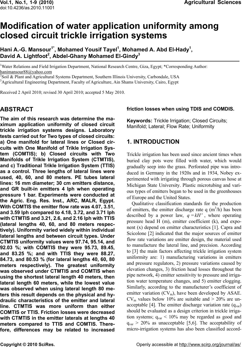
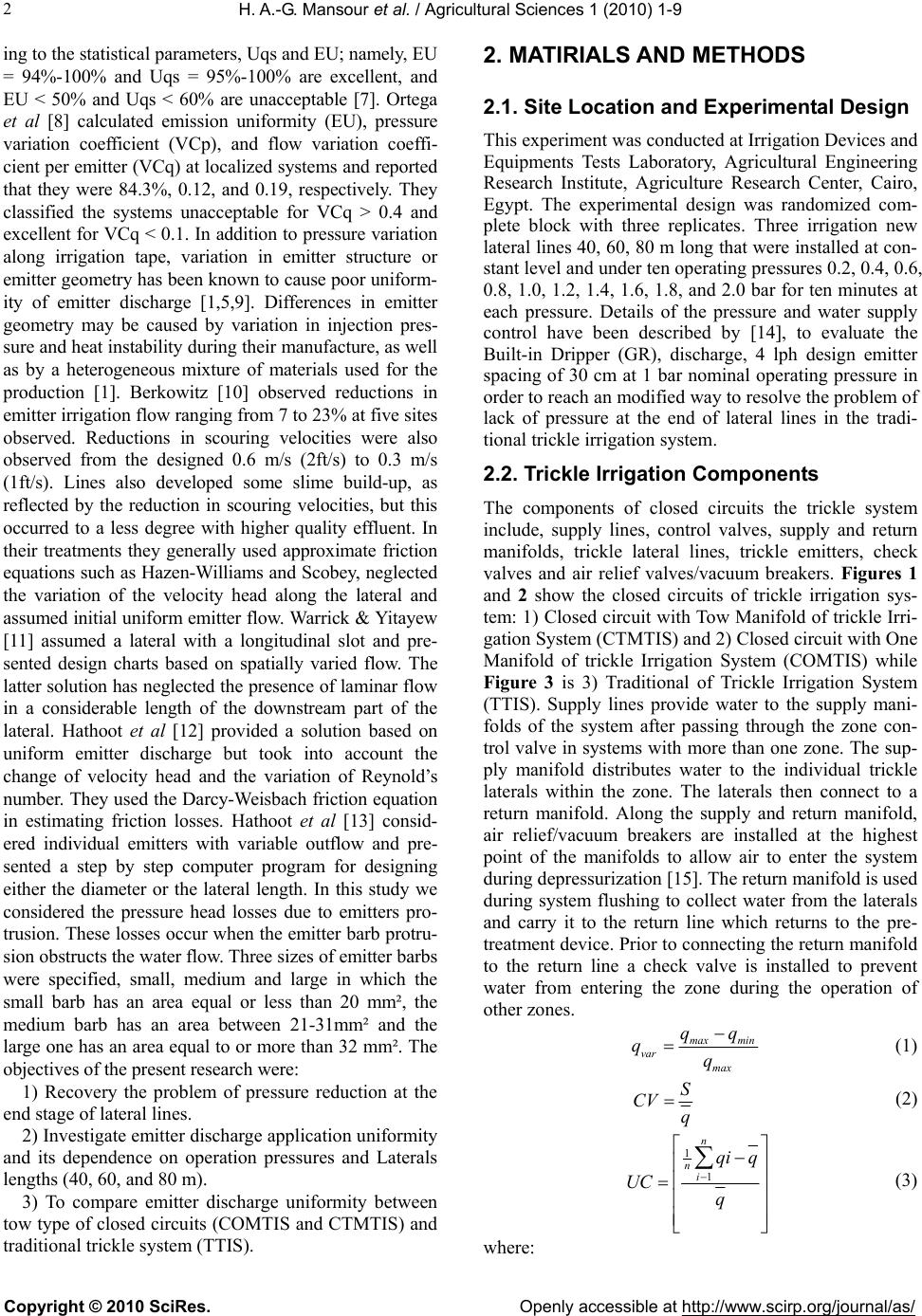
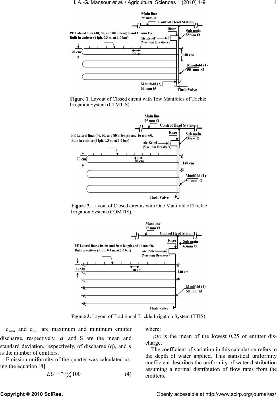
H. A.-G. Mansour et al. / Agricultural Sciences 1 (2010) 1-9

REFERENCES

[1] Kirnak, H., Doğan, E., Demir, S. and Yalçin, S. (2004)

Determination of hydraulic performance of trickle irrigation

emitters used in irrigation system in the Harran Plain.

Turkish Journal of Agriculture and Forestry, 28, 223-

230.

[2] Capra, A. and Scicolone, B. (1998) Water quality and

distribution uniformity in drip/trickle irrigation systems.

Journal of Agricultural Engineering Research, 70(4),

355-365.

[3] Mizyed, N. and Kruse, E.G. (1989) Emitter discharge

evaluation of subsurface trickle irrigation systems. Trans-

actions of the American Society of Agricultural and

Biological Engineers, 32(4), 1223-1228.

[4] American Society of Agricultural Engineers (2003) EP405.1

FEB03. Design and installation of microirrigation systems.

ASAE Standards, ASAE, St. Joseph, 901-905.

[5] Wu, I.P. and Gitlin, H.M. (1973) Hydraulics and uniformity

for drip irrigation. Journal of the Irrigation and Drain-

age Division, 99(2), 157-168.

[6] Camp, C.R., Sadler, E.J. and Busscher, W.J. (1997) A

comparison of uniformity measure for drip irrigation

systems. Transactions of the American Society of Agri-

cultural Engineers, 40(4), 1013-1020.

[7] American Society of Agricultural Engineers (1999) Design

and installation of microirrigation systems. ASAE Stan-

dards, ASAE, St. Joseph, 875-879.

[8] Ortega, J.F., Tarjuelo, J.M. and de Juan, J.A. (2002)

Evaluation of irrigation performance in localized irri-

gation system of semiaridregions (Castilla-La Mancha,

Spain). Agricultural Engineering International: The CIGR

Journal of Scientific Research and Development, 4, 1-17.

[9] Alizadeh, A. (2001) Principles and practices of trickle

irrigation. Ferdowsi University, Mashad.

[10] Berkowitz, S.J. (2001) Hydraulic performance of sub-

surface wastewater drip systems. In: Mancl, K., Ed.,

On-Site Wastewater Treatment: Proceedings of 9th Inter-

national Symposium on Individual and Small Community

Sewage Systems, 11-14 March 2001, Fort Worth, Ameri-

can Society of Agricultural Engineers, St. Joseph, 583-592.

[11] Warrick, A.W. and Yitayew, M. (1988) Trickle lateral

hydraulics. I: Analytical solution. Journal of Irrigation

and Drainage Engineering, American Society of Civil

Engineers, 114(2), 281-288.

[12] Hathoot, H.M., Al-Amoud, A.I. and Mohammed, F.S.

(1991) Analysis of a pipe with uniform lateral flow.

Alexandria Engineering Journal, 30(1), C49-C54.

[13] Hathoot, H.M., Al-Amoud, A.I. and Mohammed, F.S.

(1993) Analysis and design of trickle irrigation laterals.

Journal of the Irrigation and Drainage Division, American

Society of Agricultural Engineers, 119(5), 756-767.

[14] Perold, R.P. (1977) Design of irrigation pipe laterals.

Journal of the Irrigation and Drainage Division, American

Society of Civil Engineers, 103(2), 179-195.

[15] Netafim Irrigation, Inc. (2002) Bioline design guild.

http://www.netafim.com. Fresno, C.A. and Perkins, J.P.

(1989) On-site wastewater disposal. National Environ-

mental Health Association, Lewis Publishers, Inc., Chelsea.

[16] American Society of Agricultural Engineers (1983) Designs

and operation of farm irrigation systems. ASAE, St.

Joseph, 3, 189-232.

[17] Burt, C.M., Clemens, A.J., Strelkoff, T.S., Solomon, K.H.,

Blesner, R.D., Hardy, L.A. and Howell, T.A. (1997)

Irrigation performance measures: Efficiency and uniformity.

Journal of the Irrigation and Drainage Division, American

Society of Civil Engineers, 123(6), 423-442.

[18] Williams, G.S. and Hazen, A. (1960) Hydraulic tables.

3rd Edition, John Wiley and Sons, New York.

[19] Mogazhi, H.E.M. (1998) Estimating of Hazen-Williams

coefficient for polyethylene pipes. Journal of Trans-

portation Engineering, 124(2), 197-199.

[20] Bombardelli, F.A. and Garcia, M.H. (2003) Hydraulic

design of largediameter pipes. Journal or Hydraulic

Engineering, 129(11), 839-846.

[21] Hathoot, H.M., Al-Amoud, A.I. and Mohammed, F.S.

(1994) The accuracy and validity of Hazen-Williams and

Scobey pipe friction formulas. Alexandria Engineering

Journal, 33(3), C97-C106.

[22] Watters, G.Z. and Keller, J. (1978) Trickle irrigation

tubing hydraulics. ASAE Technical, American Society of

Agricultural Engineers, St. Joseph, 17.

[23] Dospekhov, B.A. (1984) Field experimentation statistical

procedures. Mir Publishers, Moscow, 351.

[24] Gillbert, R.G., Nakayama, F.S. and Bucks, D.A. (1979)

Trickle irrigation: Prevention of clogging. Transactions

of American Society of Agricultural Engineers, 22(3),

514-519.

[25] Khatri, K.C., Wu, I.P., Gitlin, H.M. and Phillips, A.L.

(1979) Hydraulics of micro tube emitters. Journal of

Irrigation and Drainage Engineering, American Society

of Civil Engineers, 105(2), 163-173.

[26] American Society of Agricultural Engineers (1996) EP458.

Field evaluation of microirrigation systems. ASAE Stan-

dards, 43rd Edition, ASAE, St. Joseph, 756-761.