Paper Menu >>
Journal Menu >>
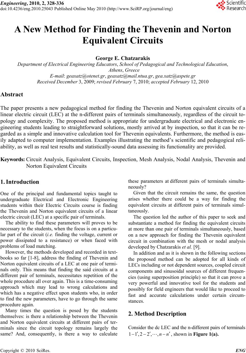 Engineering, 2010, 2, 328-336 doi:10.4236/eng.2010.25043 Published Online May 2010 (http://www.SciRP.org/journal/eng) Copyright © 2010 SciRes. ENG A New Method for Finding the Thevenin and Norton Equivalent Circuits George E. Chatzarakis Department of Electrical Engineering Educators, School of Pedagogical and Technological Education, Athens, Greece E-mail: geaxatz@otenet.gr, geaxatz@mail.ntua.gr, gea.xatz@aspete.gr Received December 3, 2009; revised February 7, 2010; accepted February 12, 2010 Abstract The paper presents a new pedagogical method for finding the Thevenin and Norton equivalent circuits of a linear electric circuit (LEC) at the n-different pairs of terminals simultaneously, regardless of the circuit to- pology and complexity. The proposed method is appropriate for undergraduate electrical and electronic en- gineering students leading to straightforward solutions, mostly arrived at by inspection, so that it can be re- garded as a simple and innovative calculation tool for Thevenin equivalents. Furthermore, the method is eas- ily adapted to computer implementation. Examples illustrating the method’s scientific and pedagogical reli- ability, as well as real test results and statistically-sound data assessing its functionality are provided. Keywords: Circuit Analysis, Equivalent Circuits, Inspection, Mesh Analysis, Nodal Analysis, Thevenin and Norton Equivalent Circuits 1. Introduction One of the principal and fundamental topics taught to undergraduate Electrical and Electronic Engineering students within their Electric Circuits course is finding the Thevenin and Norton equivalent circuits of a linear electric circuit (LEC) at a specific pair of terminals. The ability to find these parameters will proves to be necessary to the students, when the focus is on a particu- lar part of the circuit (i.e. finding the voltage, current or power dissipated to a resistance) or when faced with problems of load matching. However, the methods developed and recorded in text- books so far [1-8], address the finding of Thevenin and Norton equivalent circuits of a LEC at one pair of termi- nals only. This means that finding the said circuits at a different pair of terminals, necessitates repetition of the whole procedure all over again. This is a time-consuming approach which may lead to wrong calculations and which has a negative effect upon students who, in order to find the new parameters, have to go through the same procedure again. Many times the question is posed by the students themselves: is there a relationship between the Thevenin and Norton equivalent circuits at different pairs of ter- minals since the circuit topology remains largely the same? And, consequently, is there a way to calculate these parameters at different pairs of terminals simulta- neously? Given that the circuit remains the same, the question arises whether there could be a way for finding the equivalent circuits at different pairs of terminals simul- taneously. The question led the author of this paper to seek and substantiate a method for finding the equivalent circuits at more than one pair of terminals simultaneously, based on a new approach for finding the Thevenin equivalent circuit in combination with the mesh or nodal analysis developed by Chatzarakis et al. [9]. In addition and as it is shown in the following sections the proposed method can be adopted for all kinds of LECs including or not dependent sources, coupled circuit components and sinusoidal sources of different frequen- cies (using superposition principle) so that it can prove a very powerful and innovative tool for the students and possibly for field engineers that would like to proceed to fast and accurate calculations under certain circum- stances. 2. Method Description Consider the dc LEC and the n-different pairs of terminals nn ,,22,11 , shown in Figure 1(a). 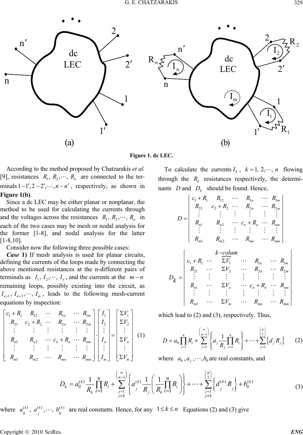 G. E. CHATZARAKIS329 )a( dc LEC 1 1 2 2 n n )b( dc LEC 1 1 2 2 n n n R n I 2 R 2 I 1 I 1 R m I Figure 1. dc LEC. According to the method proposed by Chatzarakis et al. [9], resistances are connected to the ter- minals , respectively, as shown in Figure 1(b). 12 ,,, n RR R nn ,,2 2,11 Since a dc LEC may be either planar or nonplanar, the method to be used for calculating the currents through and the voltages across the resistances in each of the two cases may be mesh or nodal analysis for the former [1-8], and nodal analysis for the latter [1-8,10]. 12 ,,, n RR R Consider now the following three possible cases: Case 1) If mesh analysis is used for planar circuits, defining the currents of the loops made by connecting the above mentioned resistances at the n-different pairs of terminals as 12 ,,, n I II, and the currents at the nm remaining loops, possibly existing into the circuit, as 12 ,, nn , m I I I, leads to the following mesh-current equations by inspection: 11 121111 21 222222 12 12 nm nm nn nnnmn mmmn mmm cR RRRIV RcRRR IV RR cRRIV RRRRI V n m n (1) To calculate the currents, flowing through the resistances respectively, the determi- nants and should be found. Hence, k I1, 2,,k k R k DD 11 1211 212222 12 12 nm nm nn nnn m mmnmm cR RRR RcRRR DRR cRR RRR R m 1111 1 2122 2 1 1 nm nm nnnn mmmn k colum cRVR R RVR DkRVcR RVR nm mm R R R which lead to (2) and (3), respectively. Thus, 11 0 11 11 1 nn n nn iji j jj ii j Da RaRdR R j 0 (2) where are real constants, and 0 ,,, j aa b 11 ()()() () 0 0 11 11 111 nn n kk k ki i j jj kjk jk jk nn ii DaRaRdR b RRR k jj 0 k (3) where are real constants. Hence, for any () ()() 0 ,,, kk j aa bnk 1 Equations (2) and (3) give Copyright © 2010 SciRes. ENG 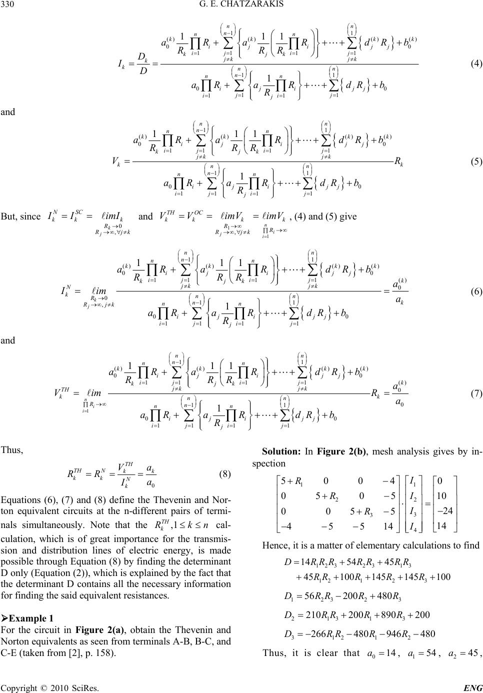 G. E. CHATZARAKIS 330 11 ()()() () 0 0 11 11 11 00 11 11 111 1 nn n nn kk k ij ijj jj ii kjk jk jk k knn n nn iji jj jj ii j aRaRdR RRR D ID aRa RdRb R k b (4) and 11 ()()() () 0 0 11 11 11 00 11 11 111 1 nn n nn kk k ij ijj jj ii kjk jk jk k k nn n nn ijijj jj ii j aRaRdRb RRR VR aRaRdRb R k (5) But, since and , (4) and (5) give kjR R k SC k N k j k imIII , 0 n ii jR k kjR R k OC k TH kimVimVVV 1 1, 11 ()()() () 0 0 11 11 () 0 011 , 00 11 11 111 1 k j nn n nn kk k ij ijj jj ii k kjk jk jk N knn Rk n nn Rjk ijijj jj ii j aRaRdRb RRRa Iim a aRa RdRb R k (6) and 1 11 ()()() () 0 0 11 11 () 0 0 11 00 11 11 111 1 n i i nn n nn kk kk ij ijj jj ii k kjk jk jk TH k k nn Rn nn iji jj jj ii j aRa RdRb RRRa Vim R a aRaRdRb R (7) Thus, 0 TH THN k kkN k Va RR a I k (8) Equations (6), (7) and (8) define the Thevenin and Nor- ton equivalent circuits at the n-different pairs of termi- nals simultaneously. Note that the cal- culation, which is of great importance for the transmis- sion and distribution lines of electric energy, is made possible through Equation (8) by finding the determinant D only (Equation (2)), which is explained by the fact that the determinant D contains all the necessary information for finding the said equivalent resistances. nkRTH k1, Example 1 For the circuit in Figure 2(a), obtain the Thevenin and Norton equivalents as seen from terminals A-B, B-C, and C-E (taken from [2], p. 158). Solution: In Figure 2(b), mesh analysis gives by in- spection 1 1 2 2 3 3 4 5004 0 05 0510 24 0055 14 45514 I R I R I R I Hence, it is a matter of elementary calculations to find 10014514510045 455414 32121 3132321 RRRRR RRRRRRRD 32321 48020056 RRRRD 200890200210 31312 RRRRD 48094648026621213 RRRRD Thus, it is clear that , , 014a154a245a , Copyright © 2010 SciRes. ENG  G. E. CHATZARAKIS331 V24 2 A B C E 3 1 4 V10 5 )a( V24 2 A B C E 3 1 4 V10 5 )b( 1 I 2 I 1 R 2 R 3 R 4 I 3 I Figure 2. Circuit for Example 1. 345a,, , and, con- sequently, (1) 056a(2) 0210a(3) 0266a 54 45 3.857 3.214 14 14 56 210 1.037A4.667A 54 45 56 210 4V 15V 14 14 TH TH AB BC NN AB BC TH TH AB BC RR II VV 45 3.214 14 266 5.911 A 45 266 19 V 14 TH CE N CE TH CE R I V Case 2) If nodal analysis is used for nonplanar circuits specifically, following a similar procedure for finding the conductance matrix determinant D, the voltages , and the currents , k V k I nk 1(as in Case 1), the following functions are always derived: 11 00 11 11 1 nn n nn iji jj jj ii j Dq GqGwGb G (9) 11 ()()() () 0 0 11 11 11 00 11 11 111 1 nn n nn kk k ij ijj jj ii kjk jk jk knn n nn iji jj jj ii j qGq GwGb GGG V qGq GwGb G k (10) 11 ()()() () 0 0 11 11 11 00 11 11 111 1 nn n nn kk k ij ijj jj ii kjk jk jk k k nn n nn iji jj jj ii j qGqGwGb GGG k I G qGq GwGb G 0 (11) where , are real constants. 00 ,,, j qq b0 () ()() ,,, j kk k qq b But, since and , (10) and (11) give 0 ,0 0 1 n ii j kG k kjG G k OC k TH kimVimVVV kjG G k SC k N k j k imIII ,0 1 11 ()()() () 0 0 11 11 () 0 00 11 00 11 11 111 1 n i i nn n nn kk k ij ijj jj ii k kjk jk jk TH knn Gn nn iji jj jj ii j qGq GwGb GGGb Vim b qGq GwGb G k (12) Copyright © 2010 SciRes. ENG  G. E. CHATZARAKIS 332 and 11 ()()() () 0 0 11 11 () 0 0, 11 00 11 11 111 1 k j nn n nn kk kk ij ijj jj ii k kjk jk jk N k k nn Gk Gjk n nn iji jj jj ii j qGqGwGb GGG b Iim G w qGq GwGb G (13) Hence, 0 b w I V RR k N k TH k N k TH k (14) Equations (12), (13) and (14) define the Thevenin and Norton equivalent circuits at the n-different pairs of ter- minals. It is worth mentioning again that calculating the is made possible through Equation (14) by finding determinant D only (Equation 9). ,1 TH k Rkn Example 2 For the circuit in Figure 3, obtain the Thevenin and Norton equivalents as seen from terminals A-B, C-B, and E-C. Solution: Since this circuit is nonplanar, the method to be used is the nodal analysis. Hence, in view of Figure 4, nodal analysis gives by inspection 8 5 5 25.15.05.0 5.04.18.0 5.08.07.1 3 2 1 33 332 1 V V V GG GGG G Hence, it is a matter of elementary calculations to find 12312 23 13 123 1.25 1.7 1.651.5 1.8751.115 1 D GGGGGGG GG GGG 12323 510.2512.15 10.05DGG G G 21313 32.2511.66.875DGGG G 31213 123 838.7 16.1 11.613.17DGGGGGGG 32 1212 810.95 16.16.295DD GGGG Thus, it is clear that , , 1 0b5.1 1w875.1 2 w 295.6 )3( 0b , , , , and, consequently, 115.1 3w05.10 )1( 0b875.6 )2( 0 b 1.5 1.875 1.5 1.875 11 10.05 6.875 10.05V6.875 V 11 10.05 6.875 6.7 A3.667A 1.5 1.875 TH TH AB BC TH TH AB BC NN AB BC RR VV II 1.115 1.115 1 6.295 6.295V 1 6.295 5.646 A 1.115 TH EC TH BC N BC R V I Case 3) By a similar procedure, the proposed method holds also for circuits containing dependent voltage and/or current sources (active circuits), as well. The A5 A B 2 2 5.2 25.1 10 A8 4 C E Figure 3. Circuit for Example 2. A5 A B 2 2 4 25.1 5.2 10 A8 1 V 2 V 3 V 2 R C 1 R 3 R E Figure 4. Method application circuit for Example 2. Copyright © 2010 SciRes. ENG 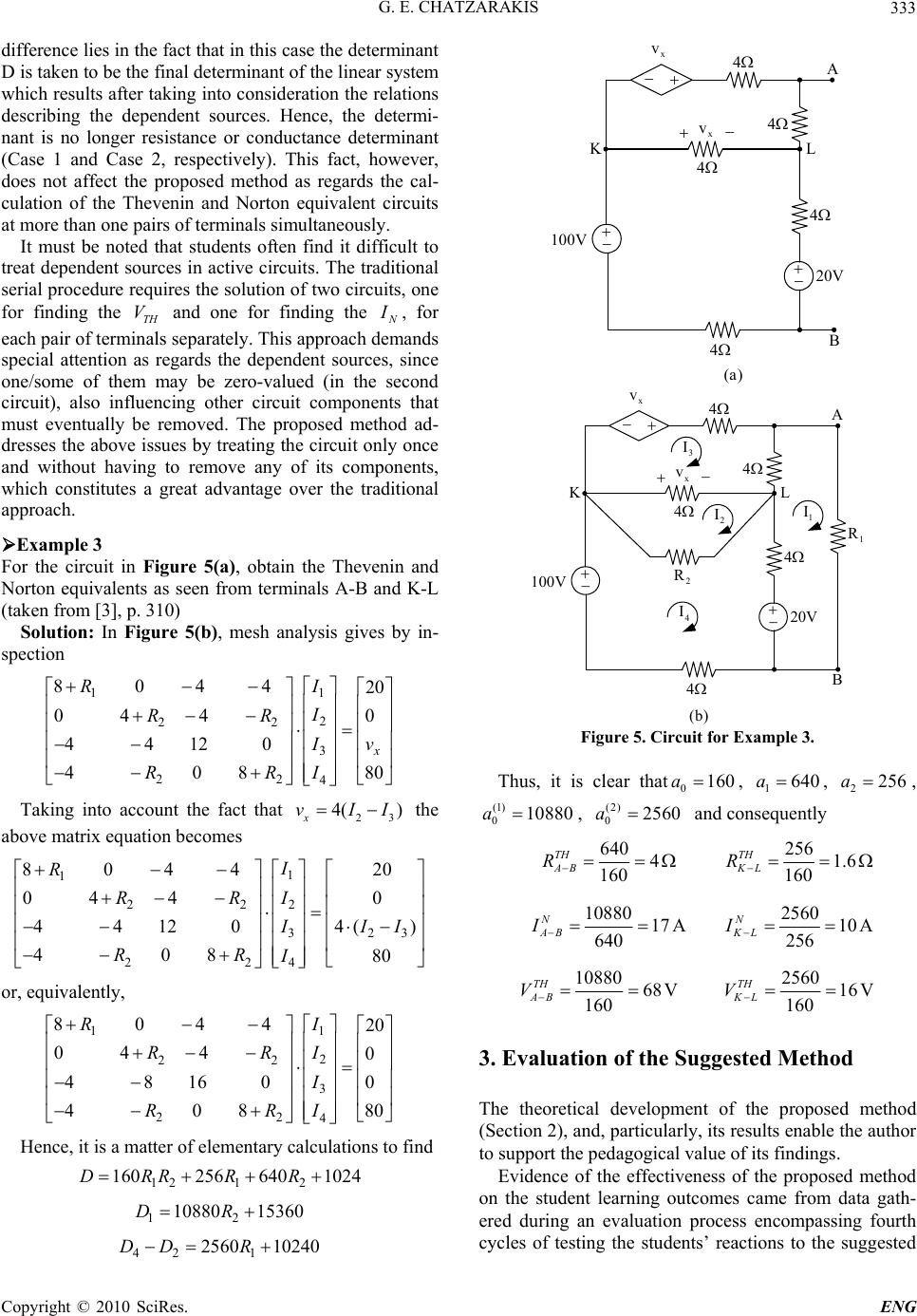 G. E. CHATZARAKIS333 difference lies in the fact that in this case the determinant D is taken to be the final determinant of the linear system which results after taking into consideration the relations describing the dependent sources. Hence, the determi- nant is no longer resistance or conductance determinant (Case 1 and Case 2, respectively). This fact, however, does not affect the proposed method as regards the cal- culation of the Thevenin and Norton equivalent circuits at more than one pairs of terminals simultaneously. It must be noted that students often find it difficult to treat dependent sources in active circuits. The traditional serial procedure requires the solution of two circuits, one for finding the and one for finding the , for each pair of terminals separately. This approach demands special attention as regards the dependent sources, since one/some of them may be zero-valued (in the second circuit), also influencing other circuit components that must eventually be removed. The proposed method ad- dresses the above issues by treating the circuit only once and without having to remove any of its components, which constitutes a great advantage over the traditional approach. TH VN I Example 3 For the circuit in Figure 5(a), obtain the Thevenin and Norton equivalents as seen from terminals A-B and K-L (taken from [3], p. 310) Solution: In Figure 5(b), mesh analysis gives by in- spection 1 1 2 22 3 22 4 8044 20 0044 44120 40880 x I R I RR v I RR I Taking into account the fact that the above matrix equation becomes 23 4( ) x vII 1 1 2 22 23 3 22 4 804420 0044 4( ) 44120 408 80 I R I RR I I I RR I or, equivalently, 1 1 2 22 3 22 4 8044 20 04 40 0 48160 80 408 I R I RR I RR I Hence, it is a matter of elementary calculations to find 12 1 2 160256 6401024DRRRR 12 10880 15360DR 421 2560 10240DD R KL 4 4 4 x v 4 4 V100 V20 A B x v )a( KL 4 4 4 x v 4 4 V100 V20 A B x v )b( 3 I 1 I 2 I 1 R 2 R 4 I Figure 5. Circuit for Example 3. Thus, it is clear that, , 0160a1640a2256a , , and consequently (1) 010880a(2) 025a60 640 256 41 160 160 10880 2560 17 A10 A 640 256 10880 2560 68 V16 V 160 160 TH TH ABK L NN ABK L TH TH ABK L RR II VV .6 3. Evaluation of the Suggested Method The theoretical development of the proposed method (Section 2), and, particularly, its results enable the author to support the pedagogical value of its findings. Evidence of the effectiveness of the proposed method on the student learning outcomes came from data gath- ered during an evaluation process encompassing fourth cycles of testing the students’ reactions to the suggested Copyright © 2010 SciRes. ENG  G. E. CHATZARAKIS Copyright © 2010 SciRes. ENG 334 Figures 6-8 show the number of students who re- sponded to each of the two methods within the allotted time, managing, at the same time, to arrive at an accurate solution in each of the 4 problem-solving situations. The outcomes show that there is a definite advantage to the proposed method as to the degree of its retention and its easy retrieval from memory, even if too much time has passed since its last exemplification and/or application (tests conducted up to 1 year later). method in comparison with the traditional serial proce- dure. The sample was taken from ASPETE, a School of Pedagogical & Technological Education, located in Athens, GR, and consisted of 4 groups of Electrical and 4 groups of Electronic Engineering students. Each group was limited to a maximum of 25 (n = 200), and there were no significant changes between cycles as to the group’s internal arrangements. The first cycle comprised six 60-minute tests, corre- sponding to the three examples examined within Cases1), 2) and 3) above, conducted 2 weeks after each method’s presentation in class (two 60-minute tests (×) three ex- amples = six 60-minute tests). It is worth noticing that the decrease rate in the num- ber of students who responded successfully in the 4 cy- cles of tests remains constant between successive tests in the case of proposed method, i.e., 175/143143/116116 / 921.2 (Figure 6) The cycle was repeated three more times (5 weeks, 1 semester and 2 semesters later), with problem-solving situations of similar complexity, and with no prior notice given to the cohorts. 132/101101/7777/ 601.3 (Figure 7) 156 /125125/100100 / 801.25 (Figure 8) 175 143 116 92 80 55 28 12 0 20 40 60 80 100 120 140 160 180 200 2 weeks la ter 5 weeks la ter 1 semester la ter 2 semesters la ter No. of Students Proposed method Classical method with serial procedure Case 1) Figure 6. Accuracy of answers with the two methods (Case 1). 132 101 77 60 68 40 20 7 0 20 40 60 80 100 120 140 160 180 200 2 weeks later5 weeks later1 semester later 2 semesters later No. of Students Proposed method Classical method with serial procedure Case 2) Figure 7. Accuracy of answers with the two methods (Case 2).  G. E. CHATZARAKIS335 156 125 100 80 44 15 41 0 20 40 60 80 100 120 140 160 180 200 2 weeks later5 weeks later1 semester later 2 semesters later No. of Students Proposed method Classical method with serial procedure Case iii) 3 Figure 8. Accuracy of answers with the two methods (Case 3). On the contrary, this rate increases significantly in the case of classical method with serial procedure, i.e., 28 /1255 /2880/551.451.2 (Figure 6) 20 / 740 / 2068 / 401.71.3 (Figure 7) 4/1 15/444/152.9 1.25 (Figure 8) Semi-structured interviews with students and teachers, administered by the author at the end of the observation cycles, cross-checked the above outcomes. The respon- dents not only validated the above findings, they also demonstrated an extremely positive attitude towards the proposed method in comparison with the traditional se- rial procedure. More particularly, students across the 8 participating groups and faculty members that were asked to apply the proposed method in their own classes appeared to have identical views regarding the fact that the proposed method “requires much less time to apply”, and that the students feel “less anxious about” and, hence, “more confident” and/or “competent” in working with it than with the traditional serial procedure. When asked to comment on the method’s effectiveness regarding stu- dent performance in terms of real test results, student and teacher comments validated qualitative impressions re- corded by the author as field notes and/or empirical data. 4. Conclusions The study presented in this paper, pertaining to the si- multaneous finding of the Thevenin and Norton equiva- lent circuits of a dc LEC at the n-different pairs of ter- minals, has led to the following conclusions: Its application by the undergraduate students of the Departments of Electrical and Electronics Engineering does not require a high level of mathematical knowledge. Basics of linear algebra pertaining to the solution of lin- ear systems could be enough. In any case, the specific subject area is included in the taught courses of first year study programs in almost all universities. It is literally applied by simple inspection, regard- less of circuit complexity and topology. This reduces the amount of anxiety experienced by the students regarding the way to the solution of the problem. Correctness of results is ensured using either calcu- lators that can treat large matrices with symbolic vari- ables or inexpensive math software for personal com- puters. Furthermore, the method is easily adapted to computer implementation. Correctness of results is also ensured by the fact that the method does not allow for an increase in the er- rors that are likely to be made from one pair of terminals to the other etc due to the repeated application of almost the same procedure. In other words the student can arrive at correct results for a number of terminals within the time period required for the calculation of these parame- ters for only one pair of terminals. Since the calculations are mostly made by inspec- tion, the students can easily apply the proposed method at a much later time than the time the specific subject area of electric circuits was taught to them. From a purely educational point of view, the pro- posed method enables the students and their instructors to calculate the said equivalent circuits at more than one pairs of terminals without having to repeat calculations right from the beginning. Hence, the approach may be said to hold a particular interest for both instructors and students, since they do not have to think and/or act de- pending on the dc LEC topology; the method leads them to an easy, systematic, time-saving and absolutely accu- rate calculation of the above parameters at more than one pairs of terminals simultaneously. We are able to know the behavior of a given circuit at any pair of terminals, with regards to the open-circuit voltage, the short-circuit current, and the equivalent re- Copyright © 2010 SciRes. ENG  G. E. CHATZARAKIS 336 sistance. This means that in theory we are able to know the pair of terminals with respect to which we may drive the maximum power the specific circuit can supply, since the matching loads are equal to the Thevenin equivalent resistances, and the voltages equal to the corresponding Thevenin voltages at every pair of terminals. In practice, however, connecting loads to a circuit is limited to specific pairs of terminals which are not many. This, in combination with the fact that the load is known, enables us to select from the few pairs of terminals the one with respect to which we may achieve the best pos- sible matching. The criterion for determining the pair of terminals where the specific load L R will be connected, is its minimum divergence from the Thevenin equivalent resistances, i.e. the appropriate pair kk , where the load connection will cause the minimum power reflec- tions, is determined by the L TH kRR min. In view of this, a major contribution of this study is the fact that in real world applications, it is very useful for the engineer to know the Thevenin equivalent circuit at more than one pairs of terminals simultaneously, in order to confront possible faults. The approach holds equally well for ac LECs, the sources of which operate at the same frequency, noting that the coefficients giving the values of the equivalent circuits parameters are all complex numbers. Finally, the accuracy and the effectiveness of the proposed method can also be verified in a laboratory environment of electric or electronic circuits where the time students spend on a weekly basis can not be very long. Following this method, students can obtain easily and fast Thevenin equivalents of multi-terminal LECs, either for practice or on purpose, that could validate the theoretic results and justify the time savings achieved. The author hopes that the reader will be inspired to re-examine his or her own text from a more critical viewpoint and perhaps add additional critical contribu- tions to the literature. The author also hopes he has ef- fectively affirmed that research (both technical and pedagogical) in circuit analysis can be both interesting and profitable. 5 . References [1] J. W. Nilsson and S. A. Riedel, “Electric Circuits,” Read- ing, Addison Wesley Publishing Company, 5th Edition, MA, 1996. [2] C. K. Alexander and M. N. O. Sadiku, “Fundamentals of Electric Circuits,” McGraw-Hill, New York, 2000. [3] G. E. Chatzarakis, “Electric Circuits,” Tziolas Publica- tions, Thessaloniki, Vol. 1, 1998. [4] G. E. Chatzarakis, “Electric Circuits,” Tziolas Publica- tions, Thessaloniki, Vol. 2, 2000. [5] W. H. Hayt and J. E. Kemmerly, “Engineering Circuit Analysis,” McGraw-Hill, New York, 1993. [6] C. A. Desoer and E. S. Kuh, “Basic Circuit Theory,” McGraw-Hill, New York, 1969. [7] R. A. Decarlo and P.-M. Lin, “Linear Circuit Analysis,” Oxford University Press, New York, 2001. [8] D.E. Johnson et al., “Electric Circuit Analysis,” Pren- tice-Hall, Upper Saddle River, 1997. [9] G. E. Chatzarakis et al., “Powerful Pedagogical Ap- proaches for Finding Thevenin and Norton Equivalent Circuits for Linear Electric Circuits,” International Jour- nal of Electrical Engineering Education, Vol. 41, No. 4, October 2005, pp. 350-368. [10] G. E. Chatzarakis, “Nodal Analysis Optimization Based on Using Virtual Current Sources: A New Powerful Pedagogical Method,” IEEE Transactions on Education, Vol. 52, No. 1, February 2009, pp. 144-150. Copyright © 2010 SciRes. ENG |