Paper Menu >>
Journal Menu >>
 International Journal of Modern Nonlinear Theory and Application, 2012, 1, 14-31 http://dx.doi.org/10.4236/ijmnta.2012.11003 Published Online March 2012 (http://www.SciRP.org/journal/ijmnta) Harmonic Analysis in Discrete Dynamical Systems Gerardo Pastor1*, Miguel Romera1, Amalia Beatriz Orue1, Agustin Martin1, Marius F. Danca2, Fausto Montoya1 1Instituto de Seguridad de la Inform ación, CSIC, Madrid, Spain 2Romanian Institute of Science and Technology, Cluj-Napoca, Romania Email: *gerardo@iec.csic.es Received February 7, 2012; revised March 9, 2012; accepted March 19 2012 ABSTRACT In this paper we review several contributions made in the field of discrete dynamical systems, inspired by harmonic analysis. Within discrete dynamical systems, we focus exclusively on quadratic maps, both one-dimensional (1D) and two-dimensional (2D), since these maps are the most widely used by experimental scientists. We first review the appli- cations in 1D quadratic maps, in particular the harmonics and antiharmonics introduced by Metropolis, Stein and Stein (MSS). The MSS harmonics of a periodic orbit calculate the symbolic sequences of the period doubling cascade of the orbit. Based on MSS harmonics, Pastor, Romera and Montoya (PRM) introduced the PRM harmonics, which allow to calculate the structure of a 1D quadratic map. Likewise, we review the applications in 2D quadratic maps. In this case both MSS harmonics and PRM harmonics deal with external arguments instead of with symbolic sequences. Finally, we review pseudoharmonics and pseudoantiharmonics, which enable new interesting applications. Keywords: Harmonic Analysis; Discrete Dynamical Systems; MSS Harmonics; PRM Harmonics; Pseudoharmonics 1. Introduction In this paper we review a branch of harmonic analysis applied to discrete dynamical systems. In general, har- monic analysis has been widely used in experimental applications, as in the field of signal processing. In the same way, harmonic analysis applied to discrete dy- namical systems can be a valuable tool for experimental scientists studying nonlinear phenomena. This paper is focused abov e all in showing some tools with interesting applications in no nl i near phenome na. At its inception, the harmonic analysis studies the rep- resentation of a function as the superposition of basic waves which, in physics, are called harmonics. Fourier analysis and Fourier transforms are the two main branches investigated in this field. The harmonic analysis is soon generalized and in the past two centuries becomes, as noted above, a wide subject with a large number of appli- cations in diverse areas of experimental science. In order to study nonlinear phenomena, experimental scientists use dynamical systems, whether continuous or discrete. In this review paper we only deal with discrete dynamical systems and more specifically with quadratic maps, above all one-dimensional (1D) quadratic maps and two-dimensional (2D) quadratic maps, which are the most commonly used. The two most popular 1D quadratic maps are the lo- gistic map 11 nnn x xx 2 and the real Mandelbrot map 1nn x xc . The logistic map [1-3] is widely known among experimental scientists studying nonlinear phenomena. Indeed, since Verhulst used it for the first time in 1845 to study populatio n growth [1 ], it has served to model a large number of phenomena. The real Man- delbrot map is the intersection of the Mandelbro t set [4-6] and the real axis. All the 1D quadratic maps are topo- logically conjugate [7-9]. Therefore, we can use one of them to study the others. The most popular 2D quadratic map is, without any doubt, the Mandelbrot set, which is the most representa- tive paradigm of chaos. The Mandelbrot set can be de- fined as :0 as k c Mc fk C, where 0 k c f is the k-iteration of the complex polynomial function depending on the parameter c, 2 c f zzc 0, z and c complex, for the initial value . In the same way as we use the Mandelbrot set to study the complex case, to study the 1D case we normally use the real Mandelbrot map [10-12] (likewise we could have used the logistic map), that can be defined again as z :0 as k rc Mc fk C , but where now 0fk c is the k-iteration of the 1D polynomial function depending on the parameter c, 2 c f xxc, x and c real, for the initial value . In this real Mandelbrot map there are several kinds of points according to the 0x *Corresponding a uthor. C opyright © 2012 SciRes. IJMNTA  G. PASTOR ET AL. 15 multiplier value d f p c x x df xx [13]. A similar definition of the multiplier λ can be given for the Man- delbrot set complex case, as can be seen for example in [6], where c is defined for the parameter values of the Mandelbrot set, which are complex values, and not only for the real values of the real segment 21c 4. In both cases, the real case and the complex one, when 1 1 one has hyperbolic points. The connected com- ponents of the c-values set for which converges to a k-cycle are periodic hyperbolic components (period i c HCs), or simply HCs [6]. These periodic HCs verify 0 k c f , which means they are stable (if 0 they are superstable). A HC is a cardioid or a disc for the complex case (2D hyperbolic components) and a segment for the real case (1D hyperbolic components). Therefore, we can speak indistinctly of periodic orbits (superstable periodic orbit if 0 ) or hyperbolic components, although in 1D quadratic maps we normally speak of periodic orbits, and in 2D quadratic maps of HCs. The variety of names is due to the fact that this paper is a review of several papers. There are also points where 1 which means they are unstable. These last points are, in addition, preperiodic and they have been later called Misiurewicz points [14-18]. When 1 one has non-hyperbolic points. These points correspond to tangent bifurcation points (or cusp points, where, in the case of a 2D quadratic map, a cardi- oid-like component is born) and to pitchfork bifurcation points (or root points, where, in the case of a 2D quad- ratic map, a disc-like component is born). Therefore in both cases, 1D and 2D quadratic maps, the two most representative elements are HCs (remember that they are more commonly called periodic orbits in 1D quadratic maps) and Misiurewicz points. There are many ways to identify both HCs and Misiurewicz points. For example, we can recognize a HC by means of its period, and a Misiurewicz point by its preperiod and period. However, normally a lot of HCs have the same period, and a lot of Misiurewicz points have the same preperiod and period; hence, this way of naming them is not uni- vocal. We are interested in names of HCs and Misi- urewicz points that can identify them univocally. When the names identify them univocally, we denominate them identifiers. As we shall see later, in 1D quadratic maps the identifiers we use are the symbolic sequences [19], which are sequences of the type CX…X (X can be a L for left, or a R for right). These sequences show the symbolic dynamics of the critical point in the map under consideration. Unfortunately, symbolic sequences can not be used as identifiers in 2D quadratic maps because two different HCs can have the same symbolic sequence. Therefore, to identify a HC (or a Misiurewicz point) in a 2D quadratic map we normally use the external argu- ments (EAs) associated to the external rays of Douady and Hubbard [15,20,21] that land in the cusp/root points of the cardioids/discs (or in the Misiurewicz points). These EAs are given as rational numbers with odd de- nominator in the case of hyperbolic components, and with even denominator in the case of Misiurewicz points. These rational numbers can also be given as their binary expansions [22], which are the most commonly used, and the only ones used here. As we shall see later, Metropolis, Stein and Stein (MSS) [23] used a variant of the harmonic analysis within the field of discrete dynamical systems, specifi- cally within a type of 1D quadratic maps, the logistic map. While in the classical harmonic analysis a function is the superposition of the infinity of its harmonics, the harmonics of MSS (MSS harmonics) of the symbolic sequence (pattern for MSS) of a superstable orbit calcu- late the symbolic sequences of the period doubling cas- cade of the original orbit. Therefore, the MSS harmonics are a very valuable tool since, given the symbolic se- quence of a superstable orbit (which characterizes the whole HC), the symbolic sequences of the infinity of orbits of its period doubling cascade can easily be calcu- lated. Indeed, if we start from a period-p orbit (or HC), the periods of the orbits calculated are 2p, 4p, 8p, … (doubling period cascade, always in the periodic region). In Section 2.1 we shall see in more detail MSS harmonics and, in addition, we also shall see MSS antiharmonics. Based on MSS harmonics and MSS antiharmonics, Pastor, Romera and Montoya (PRM) introduced in [12] Fourier harmonics (F harmonics) and Fourier antihar- monics (F antiharmonics), which in their subsequent pa- pers were simply called harmonics and antiharmonics in order to avoid confusion within the Fourier analysis. Nevertheless, if we simply call them harmonics, they can be confused with the MSS harmonics. Therefore, in this review we have called them PRM harmonics. While MSS harmonics were introduced by using the logistic map, PRM harmonics were introduced by using the real Mandelbrot map. These PRM harmonics and antihar- monics are a powerful tool that can help us in both the ordering of the periodic orbits of the chaotic region (and not only those of the periodic region as in the case of the MSS harmonics) and the calculation of symbolic se- quences of these orbits. As we shall see in more detail in Section 2.2, given the symbolic sequence of a periodic orbit, the PRM harmonics of this orbit are the symbolic sequences of the infinity of last appearance periodic or- bits of the chaotic band generated by such an orbit. As we have just said, in Sections 2.1 and 2.2 we in- troduce the harmonics/antiharmonics of MSS, and the harmonics/antiharmonics of PRM respectively, in both cases when the identifiers of the periodic orbits are the symbolic sequences corresponding to 1D quadratic maps. Copyright © 2012 SciRes. IJMNTA  G. PASTOR ET AL. 16 In Sections 3.1 and 3.2 we shall see again MSS and PRM harmonics/antiharmonics but now in 2D quadratic maps; that is, when the identifiers are EAs. When we are working in the chaotic region of 2D quadratic maps out of the period doubling cascade and out of the chaotic bands, harmonics and antiharmonics have to be generalized. That is what we do in Section 4, where pseudoharmonics and pseudoantiharmonics are introduced. These two new tools will allow new order- ings and new calculations in this chaotic region. 2. Harmonics in 1D Quadratic Maps In this section on 1D quadratic maps we first review the MSS harmonics/antiharmonics, which were introduced by MSS [23]. Given the symbolic sequence of a periodic orbit, MSS harmonics calculate the symbolic sequences of the period doubling cascade of that periodic orbit, placed in the periodic region. Finally, we review the PRM harmonics/antiharmonics [12]. Given the symbolic sequence of a periodic orbit (HC), PRM harmonics cal- culate the symbolic sequences of the last appearance pe- riodic orbits (or last appearance HCs) of that periodic orbit, placed in the chaotic region. Let us see both cases in Sections 2.1 and 2.2. 2.1. MSS Harmonics The symbolic dynamics is introdu ced by Morse and Hed- lung in 1938 [24]. According to Hao and Zhen [25], based on this theory, Metropolis, Stein and Stein [23] develop the applied symbolic dynamics to the case of one-dimensional unimodal maps, which is simpler and very useful. Applied symbolic dynamics used in the pre- sent paper is based on the paper of MSS and on the reci- pes of Schroeder [26]. The symbolic dynamics is based on the fact that some- times it is not necessary to know the values of the itera- tion but it is enough to know if these values are on the left (L) or are on the right (R) of the critical point (C). The sequence of symbols CXX…X (X is an L for left, or a R for right) is called symbolic sequence, or pattern. There are two types of 1D quadratic maps, rightward maps, R-maps, and leftward maps, L-maps [11,12]. The most representative R-map is the logistic map, n 11 nn x xx , and the most representative L-map is the real Mandelbrot map, 2 1 nn x xc . In the logistic map the critical point is a maximum, whereas in the real Mandelbrot map the critical point is a minimum. As said before, all the 1D quadratic maps are topologically con- jugate [7-9], therefore the logistic map and the real Man- delbrot map have equivalent symbolic dynamics, and the symbolic sequences of one of them can be obtained by interchanging Rs and Ls from the other one. MSS use the logistic map, an R-map, therefore the R-parity, which is the canonical parity of a R-map, has to be applied. The symbolic sequence of a periodic orbit of a R-map has even R-parity if the number of Rs is even, and it has odd R-parity if the number of Rs is odd [11,12]. Let us see now the definition of harmonic introduced by MSS. Let P be the pattern of a superstable orbit of the logistic map. The first MSS harmonic of P, 1 MSS H P, is formed by appending P to itself and changing the second C to R (or L) if the R-parity of P is even (or odd). The second MSS harmonic of P, 2 MSS H P, is formed by appending 1 MSS H P to itself and changing the second C to R (or L) if the R-parity of 1 MSS H P is even (or odd). And so on. The change from C to R or L obeys the relo rule (R if Even and L if Odd), which is the canonical rule of a R-map, and a useful mnemonic rule. As mentioned in the introduction, the periods of the successive MSS harmon- ics of a pattern P of period p are: 2p, 4p, 8p, …, which correspond to the periods of the patterns of the period doubling cascade of P. Example: We start from the period-1 superstable orbit whose pattern is C. To find the patterns of the period doubling cascade of C we have to obtain the successive MSS har- monics of C by applying the relo rule. To obtain the first MSS harmonic of C we append C to C (CC) and we change the second C to R because the R-parity of C is even. To obtain the second MSS harmonic of CR we append CR to CR (CRCR) and we change the second C to L because the R-parity of CR is odd. And so on. The results up to the fifth MSS harmonic, which correspond to the 20, 21, 22, 23, 24 and 25 periodic orbits of the period doubling cascade, are: 0CC MSS H , , , 1CCR MSS H 2C CRLR MSS H 33 CCRLR LR MSS H, 433 CCRLR LRLRLR LR MSS H, 533333 CCRLRLRLRLR LR LR LRLRLR LR MSS H i . Note that, when i = 0, M SS corresponds to the trivial case of the starting point, and only when H1, 2,i , ()i M SS H are the first, second, … MSS harmonics, respec- tively. Let us see now the definition of antiharmonics, also introduced by MSS. Let P be the pattern of a superstable orbit of the logis- tic map. The first MSS antiharmonic of P, 1 MSS A P, is formed by appending P to itself and changin g the second C to L (or R) if the R-parity of P is even (or odd). The second MSS antiharmonic of P, 2 MSS A P, is formed by appending 1 MSS A P to itself and changing the second C to L (or R) if the R-parity of 1 MSS A P is even (or odd). And so on. As can be seen, in this case the mnemonic rule is the lero rule (L if Even and R if Odd), which is the antican- Copyright © 2012 SciRes. IJMNTA  G. PASTOR ET AL. Copyright © 2012 SciRes. IJMNTA 17 onical rule of a R-map. As in the case of the MSS har- monics, the periods of the successive MSS antiharmonics of a pattern P of period p are: 2p, 4p, 8p, … Antihar- monics seem to have no interest because they do not correspond to any possible periodic orbit. However, this is not so, as we shall see later. of the symbolic sequences or patterns of superstable or- bits. However, in the same way as the Sharkovsky or- dering only treats a part of the total set of the superstable orbits, the first appearance superstable orbits, PRM only treat another part of this set, the last appearance super- stable orbits. On the other hand, while MSS or Shark- ovsky use the logistic map, a R-map, PRM use the real Mandelbrot map, a L-map, which is the intersection of the Mandelbrot set with the real axis. Example: If we start again from the period-1 superstable orbit whose pattern is C, and we calculate up to the third MSS antiharmonic by applying the lero rule, we obtain: From the introduction of PRM harmonics, PRM obtain what they call the harmonic structure of a 1D quadratic map [12], which results from the generation of all the genes, i.e., the superstable orbits of the period doubling cascade. This harmonic structure obtained from the genes is a way of seeing the ordering that clearly shows the connection between each period doubling cascade com- ponent (gene) and the corresponding chaotic band. 0CC MSS A, , 1CCL MSS A 23 CCL MSS A, , 37 CCL MSS A that indeed do not cor respond to any periodic orbit. 2.2. PRM Harmonics In 1997 the PRM harmonics and PRM antiharmonics were introduced to contribute to the ordering of 1D quad- ratic maps [12]. The search of order in chaos, and more specifically in 1D quadratic maps, was early carried out in the well known works of Sharkovsky [27,28]. Shark- ovsky’s theorem gives a clear ordering of the superstable periodic orbits but only of orbits that appear by the first time. This theorem states that the first appearance of the periodic orbits of the parameter-dependent unimodal maps are in the following universal ordering when the parameter absolute value increases: One can obtain all the structural patterns by starting out only from the pattern C of the period-1 superstable orbit. Beginning from this pattern C, all the patterns of the period doubling cascade and the patterns of the last appearance superstable orbits of the chaotic bands are generated. One can clearly see that the origin of each period- chaotic band n is the nth periodic orbit of the period doubling cascade, with period , which is the gene . 2n G B2n n 1 2 4 8 ... 2k.9 2k.7 2k.5 2k.3 ... 2.9 2.7 2.5 2.3 ... 9 7 5 3 where th e s ymbo l mu s t b e read as “precede to”. The Sharkovsky theorem gives a clear ordering of the first appearance superstable orbits (see Figure 1), but without taking into account either the symbolic sequence or the origin of each periodic orbit. On the contrary, the outstanding work of MSS [23], which also deals with the issue of ordering, uses both the symbolic sequence and the pattern generation; however, it is difficult to see any ordering there (see Figure 2, where we graphically show the MSS superstable periodic orbit generation according to the MSS theorem [23]). Figure 1. A sketch of the Sharkovsky theorem for the logis- tic map, 11 nn xxx 20p n . First appearance superstable rbits for periods As said before, PRM harmonics were introduced in [12] to better understand the ordering and the generation are shown. o Figure 2. A sketch of the successive application of the Metropolis, Stein, and Stein theorem in the logistic map 11 nn xxx n for Symbolic sequences for per iods 10p. 6p are shown.  G. PASTOR ET AL. 18 Let us consideal Ma have repeated is an L-map. As we know from [12,17], a pattern P has even L-parity if it has an even number of Ls, and has odd L-parity otherwise. L-parity is a concept similar to R-parity, introduced by MSS [23] for the logis- tic map, a R-map. Now, the definition of PRM harmonics [12,17] can be seen. Let P be a pattern. The first PRM harmonic of P, r the rendelbrot map, which as we 1 PRM H P changing the even (or 2 PRM , is formed by appending P to itself and second C to L (or R) if the L-parity of P is odd). The second PRM harmonic of P, H P, is formed by appending P to 1 PRM H P the L-parity and he second C to L (or R) if of changing t 1 PRM H P As can be is even (or odd), and so on . seen, in this case the mnem lero rule (L if Even and R if Odd), which is the canonical rule for an L-map. Application: The harmonic structure of 1D quadratic maps Let us see how to generate the chaotic bands in the real Mandelbrot map by beginning just at the origin, i.e., at the period-1 superstable orbit of symbolic sequence C. For this purpose, we shall be assisted by Figure 3, where in the upper parts we depict sketches of the PRM har- monics where periods and symbolic sequences are shown and, in the lower parts, we depict the corresponding Mandelbrot set antenna zones by means of the escape lines method [29]. Obviously, since we are in the 1D case, in these lower parts only the intersection of these figures with the real axis make sense, although we use the whole figure in order to better “see” the periodic or- bits. Let us note that, in the upper parts, symbolic se- quences corresponding to cardioids are only depicted with black half filled circles, while symbolic sequences corresponding to discs are depicted with black circles. In Figure 3(a) we show the PRM harmonics of C obtained in accordance with the lero rule. To form the first PRM harmonic of C we add a C to the C, i.e., we write CC and we change the second C into an L, since the L-parity of C is even. Therefore, the first PRM harmonic of C is . To form the second PRM harmonic of to the first one, i.e., we write CLC and we nd C into a R, since the L-parity of CL is ain the we obtain that the third and fourth PRM harmonics of C are and . As is well ], CLR, CLR (CRL, CRL2, bolic se- last appeara orbits. As it n [12,M har- cacase the the preperiod onic rule is the 1CCL PRM H C we add a C change the seco odd, and we ob t By applying 2CCLR PRM H. same procedure, 32 CCLR PRM H known [12,26 CRL3, …, in the l quences of the was already show monics of a pattern limit C PRM H is 1 and period 1, 1, 43 CCLR PRM H 2, CLR3, … ogistic map) are the sym nce superstable 30], the limit of the PR n be calculated. In this Misiurewicz point with 1 M , wnce is (CL)R (if C account, the preperiod is 2, and we have hose symbolic seque is taken into 2,1 M , as can be seen in [12]). This point is the tip (C) [1 whose parameter value is As seen in the figure, we start from the period-1 su- persta C placed in the pehe first PRMonic of C is the period-2 sble orbit of the p doubling cascade. All the oarmon- uperstable riod-20 chaotic baand are the last appeaperstable orbis . If we consider th0 supersta- gene , then the PRrmonics of the generate period-20band Howe 21able orbit n th riodrated. Let hap whendnew gene Let’ at 3(b) show harm 2,30], ble orbit harm eriod ics of C are s nd its of th ble orbit C as ne G ver, a ic regio this or onics of 2c . riodic region. T upersta ther PRM h orbits placed in the pe rance su e period-2 M ha chaotic placed i us see what 1 G. where we 0 B band a ge period- is also g bit is use 0 G the superst ene as a Figure 0 n s now look 0 B. e pe- pens the 1CLG . To form its PRonics we add Chone and we chathe second C into ordance with thrule. So, we obtain tat theond, third, anth PRM har- m , , and . The limit of these harmonics M harm nge e lero d four CLRL 1CLHG is the Misiurewicz point L to t a L or a R, h onics of 1 PRM 3 PRM e previous in acc first, sec are 1 G 1CLRLHG, 23 1 PRM HG 5 1CLRLHG 47 RL PRM 1 CLR L [16,17], that separates the and od-21 cha generom CL whic ponds to t periling casca the M harm period-21 are t appearan Agaiwe consider C PRMonics of th chaotic ba1 B (and now Figure 12, mM the peri rated f h corres od doub other PR placed in the he last n, if harm nd Let us see and fo 2 HG , placed in period-2 otic band is the pattern he secon de of th onics of C chaotic b ce supe L as a gene e gene a new 3(c) harmonics of the genee first, second, third,urth harm 89 012c 0c band 0 B 1 B. Tt harmonic C period-22, supeorbit of the dn of C. All arrstable orbits nd in addition , of this band. Gve that the gee period-21 2 G). ere the PRM 1.543 6 chaoti he firs LRL of rstable ic regio e supe 1 B and, orbits 1, we ha nerate th CLRL we show . Th d e perio L a rstable 1 ne wh G ge 2CLRLG onics of 2 G are 13 CLRLRL PRM , 3 23 CLRL 2RL PRM HG , 5 33 2 HG 7 43 CLRLRL PRM , and 2 HG the periodic region and the the period-2 is the CLRLRL PRM , the first being a new gene in others superstable orbits placed in 2 chaotic band . The limit of these harmonics Misiurewicz point 2 B 12 24,2 CLRL LRmM 1 [16,17] which separates chaotic band 2 chaotic band . Therefore the PRM harmgene period-22new gene, Figure 3(d), show PRMonics of the previous p(23) gene the period-2 2 B generate the CLRL harm 1 B chaotic band , of the next chaotic band. and the period-2 onics of the 2, and a ere we eriod-8 2 G the B wh 3 3RLG Finally, let us see Copyright © 2012 SciRes. IJMNTA  G. PASTOR ET AL. 19 stable orbits of the period doublincascade iFigure 3. A sketch of the PRM harmonics of the first four sup e PRM harmonic gener ation of last appearan chaotic band B0; (b) period-2 chaotic band B1; (c) period-4 ch 3 3CLRL RLG. A en erg n the real Man- delbrot map. Thce superstable patter ns of ctic bands is shown. (a) Pe-1 aotic band B2; (d) period-8 chaotic band B3. new period-16 ge in the periodic ted. The limit a the Miu ng cascad hao riod reg of these superst ion, 4 G, and the last appearance superstable orbits of the period-23 chaotic band 3 B are genera ble orbitsisrewicz point 1 38,4 mM [16,17] that separates the period-22 chaotic band 2 B and the period-23 chaotic band 3 B. Generalizing, the PRM harmonics of the gene n G generate the last appearance superstable orbits of the period-2n chaotic band n B, and a new gene of the period doublie, the gene 1n G is . Likewise, P RM n H G is a Misiurewicz point 1 2,2 nn n mM [10], a primary separator (or band-merging point) of the chaotic bands 1n B and n B. This double procedure (periodic orbits of the period cascade generatiodoubling chaotic band generation) contin , periodic orbits of the n and ues ifinitely and both t]. of thrhe set of the nde e co period doubling cascade onhe right and chaotic bands on the left, meet in the Myrberg-Feigenbaum point [31 Every pattern of the period doubling cascade is the responding chaotic band. Tgene PRM harmonics of all the genes is what we call the har- monic structure and is schematically shown in Figure 4. Copyright © 2012 SciRes. IJMNTA  G. PASTOR ET AL. 20 Figure 4. A sketch of the harmonic structure of the real Mandelbrot map. Each period doubling cascade superstable orbit is a gene Gn. The PRM harmonics of these genes generate the corresponding chaotic band Bn and the Misiurewicz point that separates the chaotic bands Bn–1 and Bn. The patterns of the harmonic structure are called struc- tural patterns and all of them are PRM harmonics. In Figure 4 we can see the periodic region and the chaotic region separated by the Myrberg-Feigenbaum point. Likewise, the chaotic region is divided in an infin- ity of chaotic bands B, separated by Misiurewicz points called separators, mn, . Each structural pattern of each chaotic band and each separ ator is determined by starting with the only datum of the pattern C, and by ap- As can be seen in gistic map, a R- -m t rightward ref, we have to rst Ponic of P ,1 22 nn n mM n0n plying the successive harmonics to the successive genes, what shows the power as calculation tool of the PRM harmonics. detail in [12], if we deal with the lo- map, instead of with the real Mandelbrot map, a Lap, the result is equivalent to what is shown in Figure 4. However, we haveo take into account that in this case, the canonical direction of the logistic map is the direction, the canonical parity is the R-parity and the canonical rule is the relo rule (theore interchange Ls and Rs). To finish this section, we shall see the PRM antihar- monics. Let P be a pattern. The fiRM antiharm, 1 PRM A P, is formed by ap itself and chang- pending P to ing the second C to R (or L) if the L-parity of P is even (or odd). The second PRM antiharmonic of P, 2 PRM A P, is formed by appending P to 1 PRM A P -parity of and second C to R (or L) if the Lchanging the 1 PRM A P is even M antihar- never t, although they nt role in p, to obtain (or odd). A nd s o on. As in the case of MSS an monics are also a purely correspond to a periodic orbi have no real existence, the ics. eith the lo an th tiharm form t either. B y play an gistic map, a R onics, PR al construction and u importa -ma some cases, as we shall see later. However, in the case of the structural patterns that we have treated here only PRM harmonics are present. We are dealing with the real Mandelbrot map, a L-map, and we have to apply the relo rule to obtain antiharmon- If we wre w tiharmonics we would have to apply the lero rule; that is, just the opposite than in the case of harmonics. As said before, there are two types of 1D quadratic maps, whose canonical direction are rightward for R-maps and leftward for L-maps. The canonical rule of a R-map is e relo rule, and the canonical rule of a L-map is the lero rule. Harmonics (of MSS or PRM) are obtained by apply- ing the canonical rules, and they grow in the canonical direction. Likewise, antiharmonics (of MSS or PRM) are Copyright © 2012 SciRes. IJMNTA  G. PASTOR ET AL. 21 obtained by applying the anticanonical rules, and they grow in the anticanonical direction. 3. Harmonics in 2D Quadratic Maps In the same way as in Section 2 we reviewed harmonics (both MSS harmonics and PRM harmonics) in 1D quad- ratic maps, in this section we review both types of har- monics in 2D quadratic maps. The main difference be- tween both cases is that the identifiers are the symbolic sequences for the 1D case, and the EAs (which we only use here in the binary expansion form) for the 2D case. However, in both cases, the MSS harmonics calculate the identifiers of the period doubling cascade, placed in the periodic region, and the PRM harmonics calculate the identifiers of the last appearance HCs (LAHCs), placed in the chaotic region. As said before, the 2D quadratic map used here is the Mandelbrot set, which can be seen in Figure 5(a). Let us see next MSS harmonics in Sec- tion 3.1 and PRM harmonics in Section 3.2. 3.1. MSS Harmonics For the 2D case, when we start from a period-p HC and we progress through its period doubling cascade, we find discs whose periods are 21·p, 22·p, 23·p, ... In the same way as MSS introduced the concept of harmonics in 1D y itself an bviously we unimodal maps [23], by extension we call MSS harmon- ics of a HC of the Mandelbrot set to the set constituted bd all the discs of its period-doubling cascade refer to their identifier). (oLet 12 .,.aa be the two EAs of a HC. By taking into account that the EAs of the period-2 disc are .01, .10 (see Figure 5(a)), it is easy to obtain the EAs of a MSS harmonic of 12 .,.aa from the tuning algorithm of Douady and Hubbard [21,32]. Therefore, we can define the MSS harmonics as follows: Let 12 .,.aa be the two EAs of a HC. The succes- sive MSS harmonics of the HC are given by: 012 12 .,..,. MSS H aa aa, 1121221 .,..,. MSS H aaaaaa, 21 21221 2112 .,. .,. MSS H aa aaaaaaaa , 31 21221211221121221 .,. .,. MSS H aaaa aaa aaaa aaa aaa a, … 12 .,. MSS H aa are the EAs of the Myrberg-Feigenbaum point. This notable point has neither binary nor rational EAs. Example 1 The EAs of the Mandelbrot set main cardioid are .0, .1 of the s. By applying the previous expressions, the EAs uccessive discs of the period doubling cascade of such a main cardioid can be calculated. The first MSS harmonics, up to the fourth, are: 0.0, .1.0, .1 MSS H, 1.0,.1 .01,.10 MSS H, 2.0, .1.0110,.1001 MSS H, 3.0, .1.01101001, .10010110 MSS H and 4.0, .1.0110100110010110, .1001011001101001 MSS H, as can be seen in Figure 5( a) . Example 2 If we start from the cardioid of any other midget, we can also calculate the EAs of the discs of its period dou- bling cascade. Look at Figure 5 where Figure 5(a) sws ho the Mandelbrot set; Figure 5(b) shows a sketch of the shrub (13) marked with the rectangle c in Figure 5(a); and Figure 5(c) shows the shrub (13) that is a magnify- cation of the mentioned rectangle c. Let .00111, .01000 be the EAs of the period-5 cardioid placed in the branch 11 of the shrub (13) [33] (see firstly Figures 5(b) and 5(c)). Figure 6(a) shows a magnification of the branch 11 where this period-5 representative can be better observed, and Figure 6(b) shows an additional man of such a period-5 representative. Thegnificatio EAs of the successive discs of the period doubling cascade of such a period-5 cardioid can be calculated. Calculating the MSS harmonics, up to the third, we obtain: 0.00111, .01000.00111, .01000 MSS H, 1.00111, .01000.0011101000, .0100000111 MSS , H 2.00111,.01000.00111010000100 MSS H 00 , 0111, .01000001110011101000 3.0011101000010 .00111, .01000.010 000011100111 MSS H as can be seen in Figure 6(b). Antiharmonics of MSS seem again to have no interest, as we can deduce next from th 000 eir definition: 011101000001110011101000, 0100000111010000100000111 ,…, Let 12 .,.aa be the two EAs of a HC. The success- sive MSS antiharmonics of the HC are given by: 0.,. .,. 12 12 MSS A aa aa, 1 .,..,. 212111122 2 2 .,. .,. MSS A aa aaaaaaaa,… Therefore, all of them are the same, which is the start- ing HC. 3.2. PRM Harmonics 12 1122MSS A aa aaaa, L et us see now the PRM harmonics of a HC in this 2D case. Copyright © 2012 SciRes. IJMNTA  G. PASTOR ET AL. 22 Figure 5. (a) Mandot set with the first fourelbr external argu rnal as. Shrub (1/3) is framed in rectangle c. (b) Sk in (a). (c) Shrub (1/3) that is a magnification of the rec ments of the period doubling cascade, and other significant ex- te rgumentetch o tangle c markf the shrub (1/3) corresponding to the rectangle c marked ed in (a). Copyright © 2012 SciRes. IJMNTA  G. PASTOR ET AL. 23 Figure 6. (a) Magnification of the branch 11 of the shrub (1/3) shown in Figures 5 (b) and (c), where the period-5 representa- tive can be better observed. (b) Magnification of such a period-5 representative shown in the rectangle b marked in (a), with some of its important external arguments. Let 12 .,.aa expansion be the EAs of a HC given in form of binary[22]. The EAs of the order i PRM har- monics of 12 .,.aa are given by: 121222211 1 .,. .,.. i PRM ii H aaaaaa aaaa (1) When , Equation (1) calculates a se- quence oEquati on (1) becomes: 0,1, 2, 3,i f HCs. When i, 121222211 11221 .,..,.. ,. PRM H aaaaaaaaa aaaaa (2) two preperiodic arguments, and therefore Misiurewicz points. In the 1D case, we obtained the harmonic structure through repeated application of the PRM harmonics. Similarly, in the 2D case Equation (1), applied to a given HC when 0,1, 2, 3,i f inal HC. Indeed ). By applying Eq M harmonics of G se that normally n , calculates a sequence of HCs which are the LAHCs othe corresponding chaotic band of the orig, let us analyze, as an ex- ample, the main cardioid that we consider as a gene (see Figure 7uation (1) we obtain successive PR. For we ob , a trivial cat willen into count, for 0 G the tain ac- 0 o0i be tak 0 G1i we obtain 2i we o 0. If we apply n isiurewicz point a new gene b o 1 G in e w Equation ( the regitain thLAHCs of chaotic band 2) to ain t peri- the 0 G, odic we obt on, and for B he M1,1 M , which is, is th xtrem e up- beper ee of the chaotic band 0 B. That0 G can Copyright © 2012 SciRes. IJMNTA  G. PASTOR ET AL. 24 Figure 7. The neighbourhood of the main antenna of the Mandelbrot set with three chaotic bands, B0, B1 and B2, showin g the EAs of their first LAHCs. Likewise, the main cardioid G0 and the discs of the period doubling cascade, G1, G2, ···, showing their EAs. considered the gene or generator of the chaotic band Likewise, by applying now Equation (1) to the new , we obtain, after the trivial case of , first a new in the periodic region, and tLAHCs o nd . If we apply nowtion (2 ain thsiurewicz point 0 B. gene f ) to 1 G gene 1 G 0i hen the Equa 2,1 2 G the chaotic ba , we obt1 B e Mi M , wh . That is, th 1) to ew gen ich e chaotic band ered thgene or generatoe chaot . Inneral, bying Equat a , after thial case, first a ne is the can band n G 1 upper extrem consid ge tain of the e y appl e triv 1 r of on ( B i 1 G ic gene n G be 1 B we ob in ob- ppe be n B. oni r c th band tain extre consi e peric regid then . If we a now Equa isiur oint the ge Wh we hast seen structure of the 1D case. However, since now we are in the 2D case, we only calculate the structure of the chaotic bands of the cardioid considered. Let us see two exam- ples, the first one applied to the main cardioid (see Fig- ure 7), and the second one to the period-5 midget of the branch 11 of the shrub odi n B the M m dered at on, an pply ewicz p e of the chaotic band gene or ve ju the LAHCs of the chaotic to ich . That is, e chaotic lar to the h tion (2) 1 h i n G is th n G , we e u can arm 2,2 nn M n B nerator of t is sim , wh band (13) in the chaotic region (see Figure 6(b)). Example 1 In Figure 7 we can see the neighbourhood of the main antenna of the Mandelbrot set with three chaotic bands, and , and also the main cardioid and scs ofperiod doubling cascade, …. of tod-1 main cardioid, the g, are 0 B, the d The E 1 B iAs 2 B the he peri 0 G , 2 G 0 G 1 G ene , 0.0,.1G. If Equation (1) is applied to th is main car- dioid, .0,.1 i PRM H, for 0,1,2,3,i, the sequence .0,.1 , .01, .10, .011, .100, .0111, .1000, .01111, .10000,… is obtained. The values of this sequence (without taken into account the first one) are: first the gene, and then the LAHCs of the chaotic band . If no ap- ply Equation (2), we obtain 1 G w we 0 B .0,.1 .01,.10 PRM H, a Misiurewicz point, ,101 mM , which is the upper ex- treme of consider now 0 B. Likewise, let us 1.01, .10.01,.10 PRM H as a ne w gene 1.01, .10G. By applying Equation (1) to, 1 G .01, .10 i PRM H for 0,1, 2, 3,i , we obtain the sequence .01, .10, .0110, .1001, .011010, .100101, 0, .10010101, .0110101 1010, .1001010101,… which corresponds to (after the obvious ) first the gene , and then the LAHCs of the chband If no apply Equation (2) we obtain .011010 , 1 G aotic 2 G w we1 B. .01, .10.0110,.1001 PRM H, a Misiurewicz point, ,112 mM , which is the upper extreme of B. Finally, we can consider 1 1.01, .10.0110, .1001 PRM H as a new gene 2.0110, .1001G. By applying Equation (1) to 2 G, .0110, .1001 i PRM H for 0,1, 2, 3,i, we ob- tain the sequence Copyright © 2012 SciRes. IJMNTA  G. PASTOR ET AL. 25 .0110, .1001, .01101001, .10010110, .011010011001, .100101100110, .0110100110011001, .1001011001100110, .01101001100110011001,.10010110011001100110…. After , these terms are first the gene and then th of the chaotic band . By aping Equa- tion (2ain 2 G e LAHCs ) we obt 3 G, ply 2 B .0110, .1001.01101001,.10010110 PRM H, a Misiurewicz point, ,2 , which is the upper ex- treme of B2. And so ch that, in a general case, Gn generates the chaotic band Bn (not shown in the figure). Example 2 Let us see the period-5 midget of the branch 11 of the shrub( 24 mM on, su 13) th shown in Figure 6(b) which is a magnifica- tion of e rectangle b shown in Figure 6(a). Let us con- sider this period-5 cardioid as a gene whose EAs are 0.00111, .01000G. If we apply Equation (1), 0.00111, .01000 ii PRM PRM HGH, for we obtain the sequence 0,1, 2, 3,i, .00111, .01000, .0011101000, .0100000111, .001110100001000, .010000011100111, .00111010000100001000, .01000001110011100111,…, whose terms (for ) are the LAHCs of the chaotic band . If now y Equation (2), 2i we appl 0 B .00111, .01000.0011101000,.0100000111 PRM H, a Misiurewicz point, 05,5 mM , which is both the tip of edget and the upper e void probgure. Antiharmonics of PRM neither seem to have any in- terest, as in previous cases. Indeed, according t definition: th mixtreme of 0 B. As always, we can do the same procedure in order to calculate the LAHCs of the rest of the chaotic bands. We have not done it to alems with the fi o their Let 12 .,.aa be thhe E e EAs of a HC given in form of binary expansions [22]. TAs of the order i PRM an- tiharmonics of .,.aa given by: 12 are 12 11112222 12 .,. .,..,. i PRM ii A aaaaa aaaaaaa Equation (3) b ecomes: (3) When i, 12 1111222212 .,. .,..,. A aa aaaaaaaa aa (4) The result in both equ ations is the starting HC. However, these concepts will be very useful in th e next section. 4. Pseudoharmonics and Pseudoantiharmonics in the 2D Case We have just seen that the PRM harmonics are a power- ful tool for calculating some EAs in 2D quadratic maps. However, we can go much further if we introduce an extension of these calculation tools, which we simply call pseudoharmonics and pseudoantiharmonics [35]. These new tools are applied to the EAs of two HCs, as we can see next. 4.1. Introduction of Pseudoharmonics and Pseudoantiharmonics The introduction of pseudoharmonics and pseudoanti- harmonics can be seen in detail in [35]. Let us first in- troduce pseudoharmonics. Let 12 .,.aa be the external arguments of a HC, and let 12 .,.bb be the external arguments of other HC that is related with the first one, as will be seen later. The external arguments of the order i pseudoharmonics of 12 .,.aa and 12 .,.bb are: 12121222211 1 .,. ;.,..,. i ii PHaabbabbbab bb (5) When 0,1,2, 3,i of HCs that we, Equation (5) calculates a se- quence shall determinafterwards. When e i, Equation (5) become s: .,.abab 12121222211 1 .,. ;.,..,.PHaabbabbbab bb 12 21 (6) Equation (6) calculates a pair of extern al arguments of a Misiurewicz point. Later we shall analyze th is result in every possible case. Let us now introduce pseudoant iharmoni c s. Let 12 .,.aa be the external arguents of a C, and let mH 12 .,.bb be external arguments ofther HC, that is related with the first one. The external arguments of the order i pseudoantiharmcs of e th o oni 12 .,.aa and 12 .,.bb are: Copyright © 2012 SciRes. IJMNTA 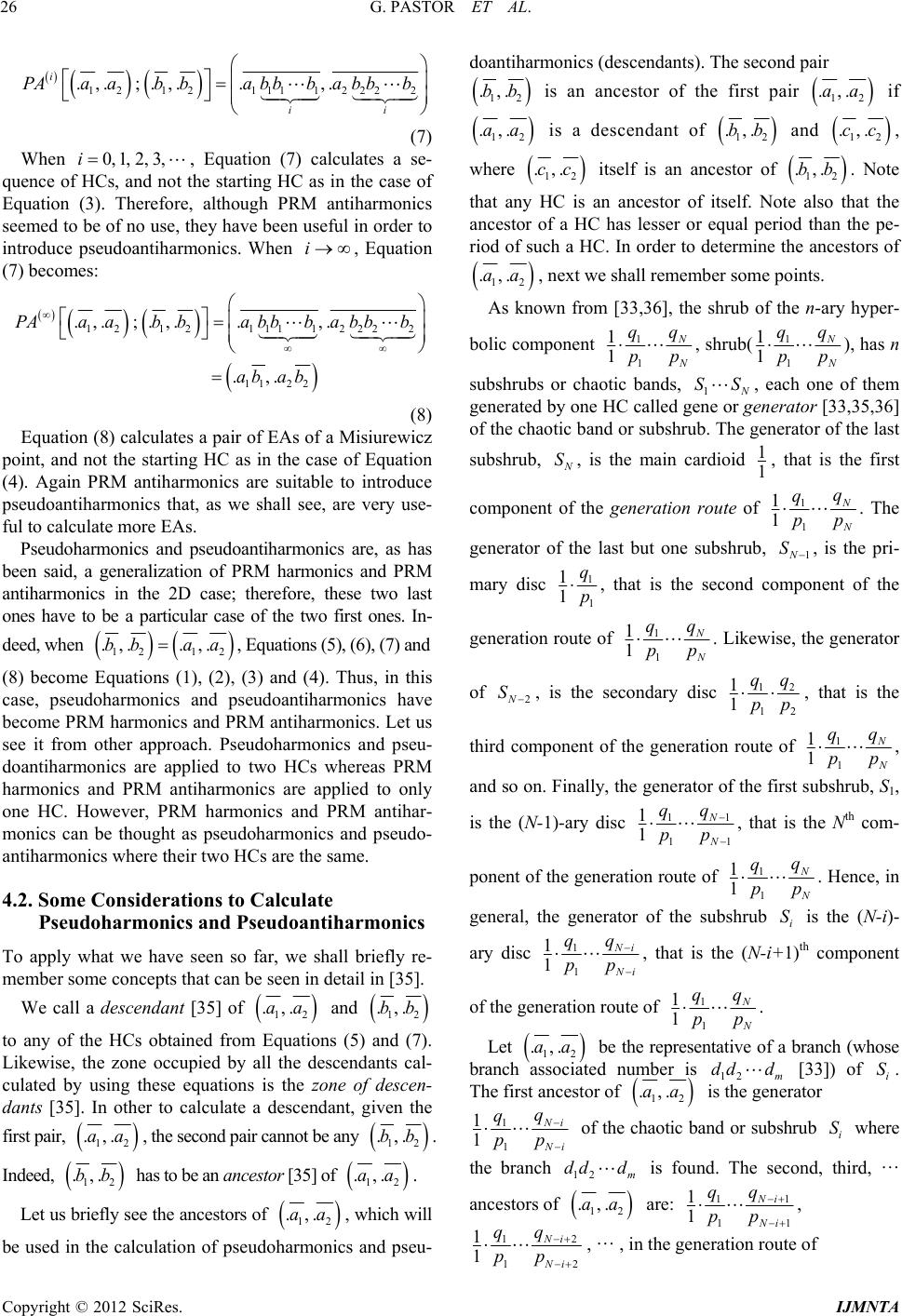 G. PASTOR ET AL. 26 121211112222 .,. ;.,..,. i ii PAaabbab bbabbb (7) When , Equation (7) calculates a se- quence and not the starting HC as in the case of Equatioe, although PRM antiharmonics seemed tey have been useful in order to introduonics. When , Equation (7) becomes: 0,1, 2, 3,i of HCs, n (3). Therefor o be of no use, th ce pseudoantiharmi 121211112222 112 2 .,. ;.,..,. .,. PAaabbab bbabbb aba b (8) Equation (8) calculates a pair of EAs of a Misiurewicz point, and not the starting HC as in the case of Equation late more EAs. ne, h av (4). Again PRM antiharmonics are suitable to introduce pseudoantiharmonics that, as we shall see, are very use- l to calcufuPseudoharmonics and pseudoantiharmonics are, as has been said, a generalization of PRM harmonics and PRM atiharmonics in the 2D case; therefortese two last ones he to be a particular case of the two first ones. In- deed, when 12 12 .,..,.bb aa, Equations (5), (6), (7) and (8) become Equations (1), (2), (3) an (4). Thus, in this case, pseudoharmonics and pseudoantiharmonics have become PRM harmonics and PRM antiharmonics. Let us see it from other approach. Pseudoharmonics and pseu- doantiharmonics are applied to two HCs whereas PRM harmonics and PRM antiharmonics are applied to only one HC. However, PRM harmonics and PRM antihar- monics can be thought as pseudharmonics and pseudo- antiharmonics where their two HCs are the same. d o 4.2. Some Considerations to Calculate Pseudoharmonics and Pseudoantiharmonics To apply what we have seen so far, we shall briefly re- member some concepts that can be seen in detail in [35]. We call a descendant [35] of 12 .,.aa and 12 .,.bb to any of the H Cs obtained from Equations (5) and (7). Lizone occupied by all the descendants cal- cu firs air kewise, the lated by using these equations is the zone of descen- dants [35]. In other to calculate a descendant, given the t p, 12 .,.aa, the second pair cannot be any 2 ,.b. Indeed, 1 .b 12 .,.bb has to be an ancestor [35] of 12 .,aa. . Let us briefly see the ancestors of .,.aa, which will be usedation oonics and pseu- 12 in the calculf pseudoharm doantiharmonics (descendants). The second pair 12 .,.bb is an ancestor of the first pair 12 .,.aa if 12 .,.aa is a descendant of 12 .,.bb and 12 .,.cc, where 12 .,.cc itself is an ancestor of 12 .,.bb. Note that any HC is an ancestor of itself. Note also that the ancestor of a HC has lesser or equal period than the pe- riod of such a HC. In order to determine the ancestors of 12 .,.aa, next we shall remember some points. As known from [33,36], the shrub of the n-ary hyper- bolic componen t 1 1 1 1 N N q q pp , shrub(1 1 1 1 N N q q pp ), has n subshrubs or chaotic bands, 1 N SS gene or , each one of them generated by one HC called generator [33,35,36] of the chaotic band or subshrub. The generator of the last subshrub, , is the main cardioid 1 N S, that is e first 1 component of the generation route of th 11 1 1 N N q q . The pp generator of the last but one suub, , is the pri- mary disc bshr 1N S 1 1 1 1 q, that is the se component of the cond p generation route of 1 1 1 1 N N q q pp . Likewise, the generator of S2N , is the secondary disc 12 12 1qq 1pp , that is the third component of the generation route of 11 11 N N q q , pp and so on. Finally, the gen subshrub, S erator of the first1, is the (N-1)-ary disc 1 1 11 1 1N pp , om- eneration roe of N q q that is the Nth c ponent of the gut11 N 1 1 N q pp . Hence, in general, the generator of the subshrubis the (N-i)- ary disc q i S 1 1 1 1 N i N i q q pp , that is the (N-i+1)th component of the generation route of 1 1 1 1 N N q q pp . Let 12 .,.aa be the representative of a branch (whose branch associated number is. The first ancestor of 12 m dd d [33]) of i S 12 .,.aa is the generator 1 1 1 1 N i N i pp q q i S where the br found. The second, third, … of the chaotic band or subshrub anch is ancestors of 12m dd d 12 .,.aa are: 1 1 1 1 1 Ni 1 N i , q q pp 2 1 1 1Ni q q pp 12Ni in the ge ne ra tion rout e of , … , Copyright © 2012 SciRes. IJMNTA  G. PASTOR ET AL. 27 1 1 1 1 N N q q pp , up to 1 1 11 1 1N N q q pp and 1 1 1 1 N N q q pp , all of them in the periodic region. Tlowing ancestors of he fol 12 .,.aa, now in the chaotic region, he repre- sentatives of the branches…, can be seen, all the ancestors oe in thbs are t . As 1 d, 12 dd , of the cha12 m dd d tic region ar Si, andere is no one in the other subshru. What we call ancestor route includes all the ordered ancestors of 12 .,.aa from the generator 1 1 1 1 N i N i q q pp to 1 1 1 1 N N q q pp in the peion, followed by the rep- resentatives of the branches 1 d, 12 dd ,…, 12m dd d in thion. riodic reg on e chaotic reg 4.3. Zes of Descendants As can be seen in detail in [35], depending on the ances- tor 12 .,.bb we shall have a different zone of descen- dants. Let us see the most important cas. es 1st case: 12 .,.bb is the first ancestor If 12 .,.aa is the representative ch of , the first ancestor of of the bran 12 m i dd dS 12 .,.aa, 12 .,.bb, is the neratorge 1 1 1 1 N i N i q q pp of5]. In this case, i S [3 12 12 .,. ;.,. i PHaabb cathe rep- resentatives of the brancheshat i an nd so on. Ob- viously, wh lculates . T 12 11 m i dd d s to say, it successively calculates first the representative of the branch 12m dd d, and then the representatives of the brches 12 1 m dd d, 12 11 m dd d, a en i one has: 1 1221 .,.. ,.PHaaabab that is the pair of external arguments the Misiurewicz point placed in the upper extreme of the branches 12 11 m dd d. Therefore, 2 12 ;.,.bb of .,. ;.,..PHaabba b 12 121221 ,.ab calculates the upper extreme of the zone of descendants of .,.aa 12 and 12 .,.bb, and 12 12 .,. ;.,. i PHaab b calculates de LAHCs in that zone. The zonendants finishes in a of desce tip or upper extreme of ; therefore, this zone of descendants cov- ers the whubshrub 2nd case: i S ole s i S. 12 .,.bb is the second ancestor, 1 1 11 1 12 .,.aa be the representative of a branch of . Since the first ancestor is 1Ni N i pp q q Let 12 m dd di S 1 1 1 1 N i N i q q pp , that is the generator of i S, the second ancestor is 1 1 11 1Ni 1 N i pp q q . Let 12 .,.bb be the external arguments of this s econd ancestor. Then 12 12 .,. ;.,.PHaab b and 12 12 .,. ;.,.PAaabb respectively calculate the upper and lower extremes of the zone of descendants of 12 .,.aa and 12 .,.bb. And, in this case, the zone of descendants is the branch 12 m dd d. On the other hand, 12 .,. ;.,. i PHaab b 12 and 12 12 .,. ;.,. i PAaab b , 0,1, 2, 3,i, respectively calculate the LAHCs i increasing and decreasing directions of the brand. 3rd case: n the ch 12m dd 12 .,.bb is the third, fourth, …, ancestor (except for the last one). Let 12 .,.aa be the representative of a branch 12 m dd d of i S. Its ancestors in the periodic region are: 1 1 1 1 N i N i q q1 1 11 1 1Ni N i q q pp pp , , 2 1 12 1 1Ni Ni q q pp , …, 1 1 1 1 N N q q pp , ancestors in the c fore, t d its anhaotic region are the representa- tives of the branches 1 d, 12 dd , …, 12 m dd d. There- he third ancestor is 2 1 1q 12 1Ni Ni q pp if we are still in the periodic region, and the representative of the branch if we are not. Now, 1 d 12 12 .,. ;.,.PHaab b and 12 12 .,. ;.,.PAaabb respectively calculate the upper and lower extremes of the zone of desce nda nts of 12 .,.aa and 12 .,.bb, that in her hand, this case is a sub-branche of dd d. On the ot 12 m 12 12 .,. ;.,.PHaab b i and 12 12 .,. ;.,. i PAaab b , 0,1, 2, 3,i, respectively calculate the LAHC decre s in the increasing and asing directions of this sub-branch of . 12 m dd d Copyright © 2012 SciRes. IJMNTA  G. PASTOR ET AL. 28 12 12 .,..,.bb aa. 4th case: As was already seen, when 12 12 .,..,.bb aa Equa- tions (5), (6), (7) and (8) become Equations (1), (2), anence pseudoha to an ely the upper extreme and the LAHCs of the chaotic band associated to any disc. 4.4. Applications Let us see an example for each of the four previous cases. Let us consider again the period-5 HC (3) d (4), hrmonics and pseudoantiharmon- ics become PRM harmonics and PRM antiharmonics. Therefore, in this case, by using pseudoharmonics and pseudoantiharmonics one can calculate the two extremes and the LAHCs of the midget associatedy cardioid, and alternativ 12 , ..00111, .01000, that is the representative the bran ch 11 of the sh rub ( .aa of 13). We help us with Figure 5, which shows such a shrub (13), and with Figure 6 whose part (a) is a magnification of the branch 11, and whose part (b) is an additional magnification of the pe- riod-5 representative. If one starts from 12 ., ..00111, .01000aa, the possible values of 12 .,.bb are, as seen before: .0,.1 and .001, .010 in the periodic region, and 11, .0100 and .00 .00111, .01000 in 1 S, that is the only subshrub of the chaotic region . 4.4.1. First Example Let us begin with 12 .,. .0,.1bb , which corresponds to the 1st case because 12 .,.bb is the generator of 1 S, and therefore the first ancestor. .00111, .01000;.0, .1.001,PH e Misiurewicz point 2,1 .010 is th M placed in the upper ex- treme of the branch 111, ftip ( 13), that is the upper extreme of the increasing part of the zone of descendants of .00111, .01000;.0, .1 , a clearly seen in s can be Figures 5(b), 5(c), and 6(a). .00111,.01000;.0, .1 i PH calculates .00111, .01000, .001111, .010000, ..0100000 , …, which arHCs in this increasing part of o 0011111, e the LA the zonef de he repre thast one i scendants, or, what is the same, tsentatives of e branches 11, 111 and 1111 (the ls not shown in the figure). In general, the increasing part of the zone of descendants starts from .,.aa, that is the repr 12 the branch dd d, and it reachesper of its chaotic band by ng the s 12 dd d only caich pseudoantiharmonics can not be used esenta- tive of the up extreme followibranche , …. This is the n 12 m 1 m, 12 dd m dd dse i12 wh11 m d, in order to calculate the decreasing part of the zone of de- scendants of .00111, .01000;.0, .1 . 4.4.2. Se Le cond Exam ple t us go on with 12 .,..001,.010bb , that corresponds to the 2nd case in w 2 .b is thncestor, 1 .,be second ahich corresponding to 1 1 1 1 N N q q pp , that in this case is the last ancestor in the periodic region. The upper and lower ex- tremes of tzone of descendants of he .00111, .01000;.001, .010 are .00111, .01000;.001, .010 0111010,.01000001 and PH .0 .001101, .00111, .01000;.001, .010 100,.01000 PA that the Misiurewicz points 5,1 M an ared 4,1 M , ex- trembranch 11 (see Figures 5(c 6(a)). As always, es of the ) and .00111, .01000;.001, .010 i PH and .00111, .01000;.001, .010 i PA calculate the LAHCs in tpart ( he increasing .00111, .01000, 00001 , .00111010, .010 .00111010010, .01000001001,…) and in the decreas- ing part ( 0, .00111001, .01000010), .00111, .0100 .00111001001, .01000010010, scendants of …) of the zone of de- .00111, .01000;.001, .010 the branch 11. 4.4.3. Third Exampl , in this case e Let us go on with 12 .,..0011, .0100bb (th3rd case e in which 12 ,. is .bbthe third ancestor). .0011, .0100 is the represef the br firsntative oanch 1, i.e. thet ancestor in the chaotic res of the zone of degion 1 S. The upper and lower extrem escendants of Copyright © 2012 SciRes. IJMNTA  G. PASTOR ET AL. 29 1000 ; .0 are .00111, .0011, .0100 .001110100,.010000011 and .00111, .01000;.0011, .0100PH .00111, .01000;.0011, .0100 .0011100,.0100001, PA that are the Misiurewicz points 5,2 M and 3, 2 M , which are the e Figure 6(a)). This sub-branch is ca xtremes of a sub-branch of the branch 11 (see lled m112 s ub dd d. Again, .00111, .01000;,.010PH .0011 0 i and 1, .01000;.0011, .0100 easing part .0011 i PA calculate the LAHCs in the incr ( .00111, .01000, .001110100, .010000011, .0011101000100, .0100000110011,…) and in the de- creasing part ( .00111,.01000, 1,.010000100 , .00111001 001011, .0100001000100,…) of the zone. 1100110 of descendan s ts of uch a sub-branch, m 112 s udbd d , although only pe If we in a case , in both cases with periods 5, 9, 13, …ri- ods 5 ane figure. where d 9 are shown in the wer 12 .,.bb is the fourth ancestlast or (but not the one), then 12 12 .,. ;.,.PHaab b and .,. ;.,.PAaabb wr and 12 12ould be the uppe lower extremes of the zone of descendants of 12 1 .,. ;.aab ichisiurewicz points that are the ex of a sub-bra 2 ,.b , wh are the M tremesnch 212 m s ubddd m of the previous sub-branch 112 s ubd dd. And so on. 4.4.4. Fourth Example Finally, let us see the nth case, that corresponds to 12 .,..00111, .01000bb , i.e. when 12 12 .,..,.bb aa. The upper and lower extremes of the zonendante of descs of .00111, .01000;.00111, .01000 are .00111, .01000;.00111, .01000 .0011101000,.0100000111 and PH .0011 .00111,.0 1000, that are the tip a to 1, .01000;.00111, .01000PA nd the cusp of the midget associated 12 12 .,..00111, .01000b, the first., .aa b one a Misiurewicz point 5,5 M and the second one the cusp of the original HC 12 .., ..00111, .01000bb 6(b)). As alwa 12 , .aa (see Figure ys, .00111, .01000;.001, .010PH i calculates the LAHCs of the increasing part of the zodants ne of descen ( .00111, .01000, .0011101000, .0100000111, .001110100001000, .010000011100111, .00111010000100001000,1110011 ,…). .0100000 110011 scendants e cusp of 5. Conclusions dratic maps, both 1D qups and 2 by experimental scientists, to this paper. vie aps, in particul h by MSS. Giverioe M the symbolic sequence of this orbit calculate the sym- bolic sequences of the period doubling cascade of the orbit. Metropolis, Stein and introducedthe first time this type of calculationand the concept of harmon- n, Pasmera and introduced the PRM harmonics. These type of harmonics the calculation band where the original orbit is. Thus, if we start froiod-1 or- bit, we can calculate the structure of a 1D quadratic map. Both, MSS harmonics and PRM ha rede- rs instead of the external argument nd the PRM ha AHCs of its chaotic Pseudoharmonics and pseudoantiharw are an expansion of PRM harmonics and PRM antiharmoni in the case of 2D quadratic maps, are a reviewed. The d make possi- This increasing part coincides with all the zone of de- scendants because the decreasing part of the zone of de- becomes a point, ththe original HC. We review a branch of the harmonic analysis applied to dynamical systems. We focus on discrete dynamical sys- tems, and more specifically on qua adratic maD quadratic maps, since these maps are the most widely used whom we have addressed We first rew the applications in 1D quadratic m ar thearmonics and antiharmonics introduced n a pedic orbit, thSS harmonics of Stein for , ics in dynamical systems. Based on MSS harmoicstor, RoMontoya expand the possibilities of s. So, given the symbolic sequence of a periodic orbit, the PRM harmonics of this orbit are the symbolic sequences of the infinity of last appearance periodic orbits of the chaotic m the pe rmonics are fined in order to can be used in 2D quadratic maps where external arguments are used as identifie symbolic sequences. Givens of a cardioid, the MSS harmonics calculate the EAs of the discs of its period doubling cascade, ar- monics the EAs of its Lband monics, cs lsose 0 B. hich new calculation tools are notably more powerful than PRM harmonics and PRM antiharmonics an Copyright © 2012 SciRes. IJMNTA  G. PASTOR ET AL. 30 ble the calculation of LAHCs inw zones of descendants. 6. on Neumann, “On Combination of Sto- inistic Processes,” Bulletin of the [3] R. M. May, “Simple M Complicated Dynamics,”0 ne Acknowledgments This work was partially supported by Ministerio de Cien- cia e Innovación (Spain) under grant TIN 2011-22668. REFERENCES [1] P.-F. Verhulst, “Recherches Mathématiques sur la Loi d’Accroissement de la Population,” Mémoires de l’Aca- démie Royale des Sciences et Belles-Lettres de Bruxelles, Bruxelles, 1844. [2] S. Ulam and J. v chastic and Determ American Mathematical Society, Vol. 53, No. 11, 1947, p. 1120. athematical Models with Very Nature, Vol. 261, 1976, pp. 459- 467. doi:10.1038/261459a [4] B. B. Mandelbrot, “Fractal Aspects of the Iteration of 1zzz for Complex and z,” Annals of the New York Academy of Sciences, Vol. 357, 1980, pp. 249-259. doi:10.1111/j.1749-6632.1980.tb29690.x [5] B. B. Mandelbrot, “O of n the Quadratic Mapping 2 zz for Complex and Frac Its μ Set, and Scaling,” D: Non nomena, Vol. 7, 1983, pp z: Thetal Structure of Physica linear Phe- . 224-239. 3)90128-8doi:10.1016/0167-2789(8 [6] B. Branner, M posia in Appa nd W. Thurston, “On Iterated Maps of the Interval,” Dynamical Systems, Vol. 1342, 1988, pp. 465- Fb0082847 “The andelbrot Set,” Proceedings of Sym- lied Mthematics, Vol. 39, 1989, pp. 75-105. [7] J. Milnor a 563. doi:10.1007/B . Jürgens and D. S New York, 1992, pp ston, 1989, pp. 44-48. omera and F. Montoya, “An Approach to the Ordering of One-Dimensional Quadratic Maps,” Chaos, l. 7, No. [8] H.-O. Peitgen, Haupe, “Chaos and Frac- tals,” Springer, . 569-574. [9] R. L. Devaney, “An Introduction to Chaotic Dynamical Systems,” Addison-Wesley, Bo [10] G. Pastor, M. R Solitons & Fractals, Vo4, 1996, pp. 565-584. doi:10.1016/0960-0779(95)00071-2 [11] M. Romera, G. Pastor, J. C. Sanz-Martín and F. Montoya, “Symbolic Sequences of One-Dimensional Quadratic Maps,” Physica A: Statistica tions, Vol. 256, No. 3-4, 1998, p 00083-1 l Mechanics and Its Applica- p. 369-382. doi:10.1016/S0378-4371(98) [12] G. Pastor, M. Romera and F. Moic Structure of One-Dimensional Quadratic Maps,” l Review E, Vol. 56, 1997, pp. 1476-1483. doi:10.1103/PhysRevE.56.1476 ntoya, “Harmon Physica [13] J. Hale and H. Koçak, “Dynd Bifurcations,” App- namics a lied Mathematics, Vol. 3, 1991, p. 314. doi:10.1007/978-1-4612-4426-4 [14] M. Misiurewicz and Z. Nitecki, “Combinatorial Patterns for Maps of the Interval,” Memoirs of the American Ma- thematical Society, Vol. 94, No. 456, 1991, pp. 109-110. [15] A. Douady and J. H., “Etude Dynamique des Polynômes Complexes,” Publications Mathematiques Hubbard 1984 (Prem ra, G. Pastor and F. Montoy a, “siurewicz P o in t s Quadratic Maps,” A: Statis- tical Mechanics and Its Applications, Vol. 232, No. 1-2, i:10.1016/0378-4371(96)00127-6 d’Orsay, 84-02, ière Partie) and 85-04, 1985 (Deuxième Partie). http://portail.mathdoc.fr/PMO/PDF/D_DOUADY_84_02. pdf http://mathdoc.emath.fr/PMO/PDF/D_DOUADY_85_04. pdf [16] M. RomeMi in One-Dimensional Physica 1996, pp. 517-535. do ra and F. Montoy ewicz Patterns in One-D A: Statist 8-4371(96)00128-8 [17] G. Pastor, M. Romea, “On the Calcula- tion of Misiurimensional Quad- ratic Maps,” Physica ical Mechanics and Its Ap- plications, Vol. 232, No. 1-2, 1996, pp. 536-553. doi:10.1016/037 [18] G. Pastor, M. Alvarez and F. Montoya, . Romera, G 292, No. 1-4, 2001, pp. 207- 230. doi:10.1016/S0378-4371(00)00586-0 “Misiurewicz Point Patterns Generation in One-Dimensional Quadratic Maps,” Physica A: Statistical Mechanics and Its Applications, Vol. [19] G. Pastor, M. Romera, J. C. Sanz-Martín and F. Montoya, “Symbolic Sequences of One-Dimensional Quadratic Maps Points,” Physica A: Statistical Mechs and Its Applications, Vol. 256, No. 3-4, 1998, pp. 369-382. doi:10.1016/S0378-4371(98)00083-1 anic [20] A. Douady and J. H. Hubbard, “Itération ds Polynômes Quadratiques Complexes,” C. R. Academic Society: Série I, Paris, 1982. Aca with External Arguments in the Mandelbrot Set Antenna,” Physica D: Nonlinear Phenome117, No. 1-2, 2002, pp. 52-71. doi:10.1016/S0167-2789(02)00539-0 e [21] A. Douady, “Chaotic Dynamics and Fractals”demic Press, New York, 1986. [22] G. Pastor, M. Romera, G. Álvarez and F. Montoya, “Op- erating na, Vol. n, “On Finite nit Interval,” Journal of Combinatorial Theory: Series A, Vol. 15, No. 1, 1973, pp. 25-44. doi:10.1016 [23] N. Metropolis, M. L. Stein and P. R. Stei Limit Sets for Transformations on the U /0097-3165(73)90033-2 [24] M. Morse and G. A. Hedl ican Journal of Mathematics, Vol. 60, No. 4, 1938, 15-866. doi:10.2307/2371264 ung, “Symbolic Dynamics,” Amer pp. 8 [25] B.-L. Hao and W.-M. Zheng, modal Maps Revisited,” Inte , Vol. 3, No. 2, 1989, pp. 235-246. 42/S0217979289000178 “Symbolic Dynamics of Uni - rnational Journal of Modern Physics B doi:10.11 der, “Fractals, Chaos, Power Laws,” W. H. Freeman, New York, 1991. Coexistence of Cycles of Continuous Line into Itself,” Ukrainia , 1964, pp. 61-71. E. Yu. Roma- adratic Maps,” Computer & [26] M. Schroe [27] A. N. Sharkovsky, “ Mapping of then Mathematical Journal, Vol. 16 [28] A. N. Sharkovsky, Yu. L. Maistrenko and nenko, “Difference Equations and Their Applications,” Kluver Academic Publishers, Dordrecht, 1993. [29] M. Romera, G. Pastor and F. Montoya, “Graphic Tools to Analyse One-Dimensional Qu Copyright © 2012 SciRes. IJMNTA  G. PASTOR ET AL. Copyright © 2012 SciRes. IJMNTA 31 Graphics, Vol. 20, No. 2, 1996,39. doi:10.1016/0097-8493(95)0013 pp. 333-3 4-4 nten [30] M. Romera, G. Pastor and F. Montoya, “On the Cusp and the Tip of a Midget in the Mandelbrot Set Ana,” Physica Letters A, Vol. 221, No. 3, 1996, pp. 158-162. [31] M. J. Feigenbaum, “Quantitative University for a Class of Nonlinear Transformations,” Journal of Statistical Phys- ics, Vol. 19, No. 1, 1978, pp. 25-52. doi:10.1007/BF01020332 [32] R. L. Devaney, “Complex Dynamical Systems,” Ameri- iden. ring,” Internation al of Bifurcation and Chaos, Vol. 13, No. 8, 2003, pp. 2279-2300. doi:10.1142/S0218127403007941 can Mathematical Society, Provce, 1994 [33] M. Romera, G. Pastor, G. Alvarez and F. Montoya, “Shrubs in the Mandelbrot Set Ordeal Journ toya, “Ex[34] G. Pastor, M. Romera, G. Alvarez and F. Mon- ternal Arguments for the Chaotic Bands Calculation in the Mandelbrot Set,” Physica A: Statistical Mechanics and Its Applications, Vol. 353, No. 1, 2005, pp. 145-158 doi:10.1016/j.physa.2005.02.025 . , V. Fernández and F. Montoya, “of Pseudoharmonics and Pseudoantiha Mathematic and Computation, Vol. 213, No. 2, 2009, pp. :10.1016/j.amc.2009.03.038 [35] G. Pastor, M. Romera, G. Alvare z, D. Arroy o, A. B. Orue A General View rmonics to Calculate External Arguments of Douady and Hubbard,” Applied 484-497. doi yo and F. ce been Subshrubs and Chaotic Bands in the Mandelbrot Set,” Disc a- [36] G. Pastor, M. Romera, G. Alvarez, D. Arro Montoya, “Equivalenetw rete Dynamics in N ture and Society, 2006, Article ID: 45920. doi:10.1155/DDNS/2006/70471 |