Circuits and Systems
Vol.07 No.06(2016), Article ID:66466,11 pages
10.4236/cs.2016.76068
Design of Robust Controller for LFC of Interconnected Power System Considering Communication Delays
T. Jesintha Mary, P. Rangarajan
Department of Electrical and Electronics Engineering, R.M.D Engineering College, Chennai, India

Copyright © 2016 by authors and Scientific Research Publishing Inc.
This work is licensed under the Creative Commons Attribution International License (CC BY).
http://creativecommons.org/licenses/by/4.0/


Received 22 March 2016; accepted 8 May 2016; published 13 May 2016
ABSTRACT
The usage of open communication infrastructure for transmitting the control signals in the Load Frequency Control (LFC) scheme of power system introduces time delays. These time delays may degrade the dynamic performance of the power system. This paper proposes a robust method to design a controller for multi-area LFC schemes considering communication delays. In existing literature, the controller values of LFC are designed using time domain approach which is less accurate than the proposed method. In proposed method, the controller values are determined by moving the rightmost eigenvalues of the system to the left half plane in a quasi-continuous way for a preset upper bound of time delay. Then the robustness of the proposed controller is assessed by estimating the maximum tolerable value of time delay for maintaining system stability. Simulation studies are carried out for multi-area LFC scheme equipped with the proposed controller using Matlab/simulink. From the results, it has been concluded that the proposed controller guarantees the tolerance for all time delays smaller than the preset upper bound and provides a bigger delay margin than the existing controllers.
Keywords:
Continuous Pole Placement Technique, Delay Margin, Delay-Dependent Stability Analysis, Frequency Sweeping Test, Load Frequency Control with Time Delays, Output Feedback Control

1. Introduction
For many years, the Load Frequency Control (LFC) plays a major role in power system operation and control. The main objective of LFC is to minimize the frequency variations when there is any change in load [1] . In traditional LFC framework, the control signals are transmitted through dedicated communication channels where the communication delays are very minimal. Nowadays, the open communication infrastructure is widely used for transmitting control signals. In such a case, time delays cannot be neglected. These time delays are certain to have an impact on the stability of the power system [2] [3] . Therefore it is essential to consider the communication delays while analyzing the stability of power system.
At present, there is a rapid momentum in the advancement of research to deal LFC with communication delays. X. Yu et al. [4] proposed a Linear Matrix Inequalities (LMI) approach for LFC system with communication delays. Hassa Bevarani et al. [5] designed a robust decentralized PI controller based on H2/H∞ control technique for three area interconnected power system with communication delay. L. Jiang et al. [6] examined the delay dependent stability of multi area LFC scheme with PI controllers using Lyapunov-theory based delay dependent criterion and LMI techniques. R. Dey et al. [7] investigated the delay dependent/independent design of H∞ controller for LFC of two area system. Chuanke Zhang et al. [8] analyzed the delay dependent stability of LFC of multi area system by finding the delay margin using LMI technique and obtaining the relationship between delay margin and controller parameter. Chuanke Zhang et al. [9] designed a PID controller for delay dependent robust load frequency control. Sahin Sonmez et al. [10] discussed about the computation of time delay margin for single area LFC system using Routh array stability criterion.
J. Chen et al. [11] presented a method to compute the delay margin of a linear time delay system by determining eigenvalues and generalized eigenvalues of certain constant matrices. The method of tracing critical eigenvalue [12] and cluster treatment of characteristics roots [13] - [15] is a direct method of finding delay margin. Another method is the indirect method to determine delay margin based on Lyapunov stability theory and LMI [16] - [18] . Wim Michiels et al. [19] suggested a new method for the determination of controller parameters in a broad class of linear control systems affected by time-delays. In this outlook, the research is focusing on designing a robust controller for LFC affected by communication delays gain prominence.
This paper proposes a new method to design a robust controller for the multi area LFC scheme considering communication delays in order to maintain the frequency and tie-line power between the areas. The controller is designed to guarantee the stability of power system for any delays smaller than the preset upper bound. The paper is organized as follows. In section 2, the multi area LFC structure is modelled considering time delays and it is represented in state space form. In section 3, the detailed description of a robust method to design the controller for multi area LFC affected by communication delays is presented. In section 4, the efficiency of the proposed controller is evaluated by computing the maximum tolerable value of time delay theoretically using Frequency Sweeping Test. In section 5, simulation is performed to prove the efficiency of the designed controller against delays for multi area LFC.
2. Dynamic Model of Multi Area LFC with Time Delay
This section illustrates the dynamic model of multi area LFC scheme with time delay. This is obtained by including an exponential term e−sτ in the secondary control loop of the conventional LFC model [1] . Figure 1 shows the block diagram of ith control area of multi-area LFC scheme where i = 1, 2…N. The exponential term denotes the time delay. The turbine, governor and generator are modelled by a first order transfer function [1] .
The notations used for ith control area are listed below.
τ transport delay.
Tgi Governor time constant.
Tti Turbine time constant.
Mi Moment of inertia of generators.
Di Damping co-efficient of generator.
Ri Speed droop.
ACEi Area Control Error.
Δfi Deviation in frequency.
ΔPtie Tie-line power flow.
ΔPti Turbine power output.
ΔPgi Governor output.
βi Frequency bias factor.
ΔPdi Total demands in area i.
Tij Synchronizing coefficient between area i and area j.

Figure 1. Dynamic model of ith control area of multi area LFC scheme.
The two-area LFC scheme with time delay can be expressed in state space form as
 (1)
(1)
 (2)
(2)
where x(t) is state vector and the state variables are  and
and  . y(t) is output vector, The output variables are
 . w(t) is disturbance vector. The disturbance variables are
 . The frequency deviations and tie line power exchange are combined together as a single variable called Area Control Error signal (ACE).
The ACE signal of area i is expressed as
 (3)
(3)
The ACE signal is used as the input to load frequency controller, which is designed as
 (4)
(4)
The closed loop model of two area LFC system can be obtained by modifying Equation (1) using state output feedback method and expressed as
 (5)
(5)
 (6)
(6)
where
 ;
; ;
; ,
,
 ;
; ,
,
 ;
; ,
,
 ,
,  ;
; 
K1 and K2 denote the gain values of PI controller. The controller values are determined using Continuous Pole Placement method which is described in detail in the next section.
3. Controller Design Based on Continuous Pole Placement Method [20]
3.1. Description of the Algorithm
The idea behind the proposed stabilization method is to move the unstable eigenvalues to the left half plane in a quasi-continuous way by applying small changes to the controller gain, in the meanwhile monitoring the other eigenvalues with a large real part. The proposed stabilization method is based on the Theorem given in Appendix 1.
The algorithm for the proposed method is as follows:
Step 1. Initialize the number of rightmost eigenvalues m = 1.
Step 2. Compute the rightmost eigenvalues for a particular preset upper bound of delay.
Step 3. Find the sensitivity of the m rightmost eigenvalues with respect to the changes in the controller gain K.
Step 4. Using the sensitivities computed in step 3, shift the m rightmost eigenvalues in the direction towards the left half plane by applying small changes to the controller gain K.
Step 5. Meanwhile monitor the uncontrolled eigenvalues. Stop when the stability is reached or go to step 2.
The detailed explanation about the different steps involved in the algorithm is presented in the following sections.
3.2. Computation of the Rightmost Eigenvalues
In 1999, Engelborghs and Roose proposed a method which computes the rightmost eigenvalues of the characteristic equation. In this method, a discretization of the time integration operator of the linearized system is obtained. The eigenvalues of the linearized system are exponential transforms of the roots of the characteristic equation. Then, the selected eigenvalues of the resulting large matrix are computed. A step length heuristic is applied to ensure that all eigenvalues are approximated accurately by discretization and the accuracy is improved by employing Newton iteration on the characteristic equation taking the approximate eigenvalues as starting values. This method is implemented in the Matlab package DDE-BIFTOOL. This package is a collection of matlab routines used to find the right most eigenvalues of the system.
3.3. Sensitivity of Eigenvalues with Respect to the Controller Gain K
The characteristics equation of the two area LFC system Equation (5) can be written as
 (7)
(7)
 (8)
(8)
where λi is a solution of the characteristic equation and n(vi) is a normalizing condition. Differentiating the Equation (7) and Equation (8) w.r.t. a component kj of K,
 (9)
(9)
From Equation (9),  and
and  can be obtained. ej is jth unity vector.
  denotes the sensitivity of the eigenvalues with respect to changes in feedback gain k.
3.4. Continuation of Eigenvalues as a Function of the Feedback Gain K
It is assumed that m eigenvalues  are to be controlled. The sensitivity of the eigenvalues with respect to changes in feedback gain is denoted as the sensitivity matrix
  where
where . The desired displacement of the controlled eigenvalues
  can be expressed as
 (10)
(10)
From Equation (10) the small changes in gain  can be calculated
 (11)
(11)
 is the Moore-Penrose inverse of sensitivity matrix (Sm). Thus with the availability of
  and
and , the small adjustments in feedback gain can be obtained one constraint that is imposed on the feedback gain is that its components must be real, but this can be obtained only by taking the components of
  in complex conjugate pairs. For the new feedback gain
 , the displacement of the controlled eigenvalues is not equal to
 , because Equation (10) is based on linearization, and some correction is required. Since the eigenvalues and eigen functions are continuous with respect to parameter changes, the predictor
 (12)
(12)
for few Newton iterations on Equation (7) are required when  is small. Since the research focuses on designing a controller in stability point of view, it is sufficient to control only the real parts of the eigenvalues i.e.,
sup . The real parts of the rightmost eigenvalues are adjusted in order to shift the rightmost eigenvalues to LHP. Therefore Equation (11) is modified as,
 (13)
(13)
where  is the desired displacement of the real parts of the controlled eigenvalues. To illustrate the
movement of the real parts of the rightmost eigenvalues of two area LFC scheme for the preset upper bound delay 4s, Figure 2 is shown.
Here the rightmost unstable eigenvalues whose real part is positive are shifted to negative real axis. The proposed algorithm converges to an optimum value at iteration on 142. At iteration 142 all the rightmost eigenvalues are moved to LHP. The final value of controller gain is K1 = [−0.0233, −0.0146]T, K2 = [0.0127, −0.0335]T. The spectrum of eigenvalues for final value of the controller gain is depicted in Figure 3.
The proposed controller guarantees the stability for the delays smaller than the preset upper bound. The robustness of the controller is validated by finding an index called delay margin. The delay margin of the system is defined as the maximum tolerable value of time delay after which the system goes unstable. The delay margin of the system is computed using Frequency Sweeping Test which is discussed in the next section.

Figure 2. Illustration of the movement of the real parts of the rightmost eigenvalues for each iteration.

Figure 3. Rightmost eigenvalues for the feedback gain (K1 = [−0.0233, −0.0146]T , K2 = [0.0127, −0.0335]T at iteration 142).
4. Computation of Delay Margin
4.1. Frequency Sweeping Test (FST)
Frequency sweeping Test [2] is applied to analyze the asymptotic stability of the system and determine the value of delay margin. The stability of the system exists only for a subset of nonnegative delays. The necessary and sufficient condition for delay-dependent stability of the system is based on the following theorem.
Let  be the delay margin. It is assumed that the system is stable at τ = 0. The rank of matrix Ad is k. The delay margin can be defined as
 (19)
(19)
where .
.
That is, the system remains stable for all  and the system becomes unstable at τ = τd. The explanation for the above theorem is presented below
The generalized eigenvalues of the matrix pencil  is calculated for various frequencies.
The generalized eigenvalues of the matrix pencil  becomes one at
 . There exists a pair (
 ,
, ) at which the absolute value of each eigenvalue variation reaches one such that delay margin
  can be obtained.
For time delay , the
, the  and
and  . Then the system remains stable.
At  the
the  and
and . Then the system goes unstable.
4.2. Algorithm for Delay Margin Calculation
The algorithm of Frequency sweeping Test for computing the delay margin is given below:
1) Obtain the maximum of real parts of all eigenvalues of the matrix A + Ad. If it is less than zero proceed.
2) Find the rank of matrix Ad. Consider rank(Ad) = k. then the number of crossover points from right half plane to left half plane is k.
3) Choose the frequency range and step size of frequency range.
4) For different frequencies , find the absolute values of all the eigenvalues of the matrix pencil
 .
.
5) Determine the angle and frequency at which the absolute value of each eigenvalue variation reaches one. Otherwise go to step 3 and vary the frequency range.
6) Calculate the delay margin 
where .
.
5. Case Study
Simulation studies have been carried out for multi- area LFC equipped with PI controller assuming the load change of 0.1 p.u in Area 1. The system parameters of each control area are listed in Table 1.
The upper bounds of time delay in each area are preset as same value while designing the controllers. First the controller values are determined by using continuous pole placement method and then for the designed controller values, delay margin is theoretically calculated using FST. The theoretical results are presented in Table 2.
The theoretical value of delay margin is calculated as 34.612 s. That is, the controller designed using the proposed method for the preset upper bound of delay 8 s not only retains stability for time delays up to 8s, it can also ensure stability till 34.612 s (delay margin). To validate the theoretical results, simulation is performed using MATLAB/SIMULINK by increasing the delay step by step from zero until the LFC system becomes unstable. The simulation results are shown in Figure 4 from which it is observed that the delay margin of the system is 34.6 s which is very closer to the theoretical delay margin (34.612).
Similarly, the controller values of three-area LFC are determined using the proposed method for preset upper bound of time delay 10 s. The results are compared with the controller gain reported in [9] and shown in Table 3.
The delay margin of the three-area LFC system with PI controller (designed using proposed method) is theoretically computed as 21.115 s whereas the method reported in (9) can maintain the stability only up to 14 s. This

 (a) (b)
Figure 4. Frequency deviation of two area LFC for preset time delay 8s. (a) Area 1, (b) Area 2.

Table 1. System parameters.
Table 2. Controller parameters of two area LFC system or preset upper bound of time delay 8 s.
clearly shows that the proposed controller is highly robust compared to the existing method.
To validate the theoretical delay margin values, simulation is performed for three area LFC scheme keeping the preset upper bound of time delay as 10 s and the results are shown in Figure 5. The solid line shows the response of system for preset upper bound of delay 10 s and dashed line shows the response of the system for delay margin. The simulation results reveal that, the stability of the system is guaranteed for all time delays smaller than the delay margin. From the figure, it can be concluded that the delay margin of the system is 21.1s which is nearer to the theoretical delay margin 21.115 s.
 (a)
(a)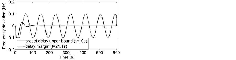 (b)
(b) (c)
(c)
Figure 5. Frequency deviation of three area LFC for preset time delay 10 s. (a) Area 1, (b) Area 2, (c) Area 3.
Table 3. Controller parameters of three area LFC system for preset upper bound of time delay 10 s.
6. Conclusion
In this paper, a robust controller based on continuous pole placement method is designed for multi area LFC scheme affected by communication delays. The controller values are determined by shifting the rightmost eigenvalues to left half plane in a quasi continuous way for any particular preset upper bound of time delay. The proposed controller is highly robust in sustaining the stability of the system even for delays greater than the preset upper bound of time delay. Case studies have been carried out for two area and three area LFC schemes. The efficiency of the controller is validated by finding the value of time delay margin theoretically using Frequency Sweeping test. The theoretical value of delay margin is verified using simulation studies. Simulation result shows that the proposed controller gives larger stability margin.
Cite this paper
T. Jesintha Mary,P. Rangarajan, (2016) Design of Robust Controller for LFC of Interconnected Power System Considering Communication Delays. Circuits and Systems,07,794-804. doi: 10.4236/cs.2016.76068
References
- 1. Kundur, P. (1994) Power System Stability and Control. McGraw-Hill Inc., New York.
- 2. Gu, K., Kharitonoy, V.L. and Chen, J. (2003) Stability of Time Delay Systems. Birkh?user, Boston.
http://dx.doi.org/10.1007/978-1-4612-0039-0� - 3. Niculescu, S.I. (2001) Delay Effects on Stability—A Robust Control Approach. Springer-Verlag, New York.
- 4. Yu, X.F. and Tomsovic, K. (2004) Application of Linear Matrix Inequalities for Load Frequency Control with Communication Delays. IEEE Transactions on Power Systems, 19, 1508-1515.
http://dx.doi.org/10.1109/TPWRS.2004.831670 - 5. Bevarani, H. and Hiyama, T. (2009) On Load-Frequency Regulation with Time Delays: Design and Real Time Implementation. IEEE Transactions on Energy Conversions, 24, 292-300.
http://dx.doi.org/10.1109/TEC.2008.2003205 - 6. Jiang, L., Yao, W., Wu, Q.H., Wen, J.Y. and Cheng, S.J. (2012) Delay-Dependent Stability for Load Frequency Control with Constant and Time Varying Delays. IEEE Transactions on Power Systems. 27, 932-941.
http://dx.doi.org/10.1109/TPWRS.2011.2172821 - 7. Dey, R., Ghosh, S., Ray, G. and Rakshit, A. (2012) H∞ Load Frequency Control of Interconnected Power Systems with Communication Delays. International Journal of Electrical Power & Energy Systems, 42, 672-684.
http://dx.doi.org/10.1016/j.ijepes.2012.03.035 - 8. Zhang, C.K., Jiang, L., Wu, Q.H., He, Y. and Wu, M. (2013) Further Results on Delay Dependent Stability of Multi Area Load Frequency Control. IEEE Transactions on Power Systems, 28, 4465-4474.
http://dx.doi.org/10.1109/TPWRS.2013.2265104 - 9. Zhang, C.K., Jiang, L., Wu, Q.H., He, Y. and Wu, M. (2013) Delay Dependent Robust Load Frequency Control for Time Delay Power System. IEEE Transactions on Power Systems, 28, 2192-2201.
http://dx.doi.org/10.1109/tpwrs.2012.2228281 - 10. Sonmez, S., Ayasun, S. and Eminoglu, U. (2014) Computation of Time Delay Margins for Stability of a Single Area Load Frequency Control System with Communication Delays. WSEAS Transactions on Power Systems, 9, 67-76.
- 11. Chen, J., Gu, G. and Nett, C.N. (1995) A New Method for Computing Delay Margins for Stability of Linear Delay Systems. System and Control Letters, 26, 107-117.
http://dx.doi.org/10.1016/0167-6911(94)00111-8 - 12. Jia, H.J. and Yu, X.D. (2008) A Simple Method for Power System Stability Analysis with Multiple Time Delays. Proceedings of IEEE Power and Energy Society General Meeting—Conversion and Delivery of Electrical Energy in the 21st Century, Pittsburgh, 20-24 July 2008, 1-7.
- 13. Olgac, N. and Sippahi, R. (2002) An Exact Method for Stability Analysis of Time Delayed Linear Time Invariant (LTI) Systems. IEEE Transactions on Automatic Control, 47, 793-797.
- 14. Sippahi, R. and Olgac, N. (2005) Complete Stability Robustness of Third-Order LTI Multiple Time-Delay Systems. Automatica, 41, 1413-1422.
http://dx.doi.org/10.1016/j.automatica.2005.03.022 - 15. Liu, Z.Y., Zhu, C.Z. and Jiang, Q.Y. (2008) Stability Analysis of Time Delayed Power System Based on Cluster Treatment of Characteristics Roots Method. Proceedings of IEEE Power and Energy Society General Meeting—Con- version and Delivery of Electrical Energy in the 21st Century, Pittsburgh, 20-24 July 2008, 1-6.
- 16. He, Y., Wang, Q.G., Xie, L.H. and Lin, C. (2007) Further Improvement of Free-Weighting Matrices Technique for Systems with Time Varying Delay. IEEE Transactions on Automatic Control, 52, 293-299.
http://dx.doi.org/10.1109/TAC.2006.887907 - 17. Wu, M., He, Y., She, J.H. and Liu, G.P. (2004) Delay Dependent Criterion for Robust Stability of Time Varying Delay Systems. Automatica, 40, 1435-1439.
http://dx.doi.org/10.1016/j.automatica.2004.03.004 - 18. Xu, S.Y. and Lam, J. (2007) Equivalence and Efficiency of Certain Stability Criteria for Time-Delay Systems. IEEE Transactions on Automatic Control, 52, 95-101.
http://dx.doi.org/10.1109/TAC.2006.886495 - 19. Michiels, W., Vyhlidal, T. and Zitek, P. (2010) Control Design for Time-Delay Systems Based on Quasi-Direct Pole Placement. Journal of Process Control, 20, 337-343.
http://dx.doi.org/10.1016/j.jprocont.2009.11.004 - 20. Michiels, W., Engelborghs, K., Vansevenant, P. and Roose, D. (2002) Continuous Pole Placement for Delay Equations. Automatica, 38, 747-761.
http://dx.doi.org/10.1016/S0005-1098(01)00257-6
Appendix 1
Lemma.
Let f(λ) and the sequence {fn(λ)}n≥1 be analytic functions on an (open) domain D ⊆ C. Suppose that {fn(λ)}n≥1 converges uniformly to f(λ) on the disc  for some R>0 and that on this disc
 is the only zero of f(λ); with multiplicity k≥0 (k = 0 means no zeros in D). Then there exists a number N ∈ N such that ∀n≥N; fn(λ) has exactly k zeros
  in D and limn→∞λn,j = λ0;
 .
.
With this lemma, continuity properties of the spectrum with respect to the feedback gain K can easily be deduced.
Theorem. For the system  the individual eigenvalues are continuous with respect to changes in the controller gain K. Moreover
  is continuous w.r.t. K.