Journal of Modern Physics
Vol.4 No.1(2013), Article ID:27250,17 pages DOI:10.4236/jmp.2013.41018
On Dynamics in a Quasi-Measurement Field
National Aeronautics and Space Administration, Johnson Space Center, Houston, USA
Email: robert.l.shuler@nasa.gov, mc1soft@yahoo.com
Received October 31, 2012; revised November 30, 2012; accepted December 8, 2012
Keywords: Inertia; Gravity; Quantum; Measurement; Relativity; Uncertainty; Equivalence; Dark Energy
ABSTRACT
A general theory of inertia tends to be circular because momentum and therefore inertia are taken as assumptions in quantum field theories. In this paper we explore instead using position uncertainty to infer inertia with mediation by quasi-measurement interactions. This method avoids attachment to the reference frame of the source masses and is thus completely relativistic, overcoming a conflict between historical theories of inertia and relativity. We investigate what laws of motion result, and whether natural explanations for equivalence and dark energy emerge.
1. Introduction
Quantum field theories have had outstanding success in explaining three of the four basic forces by means of energy fields, which when quantized, yield bosons that mediate force interactions. But the application of quantum field theory to gravity is not straightforward because of the universality of gravity (the problem of equivalence) and because gravity theories employ Riemannian curved space-time (the problem of background independence). In this paper we examine a quantum field based on position rather than energy in which mediating interactions are measurement-like and arise from position uncertainty. This is, as opposed to momentum-like arising from energy uncertainty.
While General Relativity Theory (GRT) assumes the equivalence of inertial and gravitational mass, and derives the inertial path of an object as a geodesic in a space-time metric, the inertial resistance to deviation from that geodesic still relies upon the assumption of Newton’s Law of Motion, . Standard quantum field theories yield forces based on relative position, not acceleration, except in the special case of the Higgs field which provides inertial mass for W and Z bosons. There have been some esoteric attempts to define a general field theory of inertia, but such a theory remains largely an open question.
Metric theories of gravity, those such as GRT which are based on Riemannian curvature of space-time, are widely thought to be the only viable way to satisfy the Equivalence Principle. A great deal of work has been done to experimentally verify the Equivalence Principle from the time of Galileo onward. However, the necessity of a metric theory of gravity in connection with equivalence remains a convincing argument and not a rigorous theorem [1]. There may be alternative ways to satisfy the Equivalence Principle, yet not be a pure metric theory [2].
What constitutes a metric theory? In the strict sense, superstring theory is not metric, because of residual coupling of gravitation-like fields to matter [1]. In the theory presented herein there is no gravitational field, or force, but uncertainty must be considered together with the space-time metric to determine trajectories, and there is a linkage of time and uncertainty with a field that determines inertia and indirectly gravity. If one measures distance with light path delay, the theory has non-Euclidean time and space, and excess radius near gravitating objects and is clearly metric. But in the way that the theory measures distance, it has non-Euclidean time and spatial uncertainty, and might be described as “metric-like”.
It is well known that time is dilated in a gravitational field. Time dilation implies a corresponding velocity decrease, as the parts of a clock slow down. These changes can be linked to inertia, which as measured by a remote observer increases in proportion to time dilation in connection with conservation of momentum. Numerous investigators have noted that inertia is proportional to gravitational potential, including Einstein [3,4], Sciama [5], Davidson [6], and Ciufolini and Wheeler [7].
In the reference frame of an object, using the object’s proper time, the inertia increase effect is not observable. As is well known from Special Relativity Theory (SRT), the time dilation exactly matches inertia increase. It is only a difference of inertia between reference frames, corresponding to a difference of potential, which is observable. Thus when Brans argued that all effects of the metric of GRT on inertia could be “transformed away” in a sufficiently small reference frame [8], the point of potential difference was dismissed.
However, there is circularity to basing inertia on potential. Potential is energy, and inertia is energy, so potential is (or has) inertia (or mass). We cannot really use potential as a starting point. Neither can we use momentum, since momentum includes an inertia component, and in fact we cannot use force either, since a force is equivalent to a series of momentum impulses, as for example in a quantum field. Without force, mass or potential, it seems unlikely we should be able to use the general notion of energy, either. What then?
In a conventional quantum field, particles which have sufficiently definite position such that they cannot interact directly without implying action at a distance, can interact via the field. The field conveys momentum via interactions with virtual particles, which are allowed by the uncertainty in energy. Since in explaining inertia we must also explain momentum and energy, we will look at a different aspect of uncertainty, the uncertainty of position. This degree of uncertainty may allow particles to overlap in position and interact directly. The interaction that they have may be more akin to measurement, and instead of conveying momentum, it may convey information about position and thereby mass.
2. Uncertainty and Mass
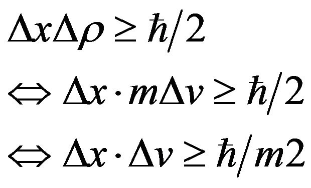
Consider the uncertainty principle in the form
 (1)
(1)
If a mass is differentially small (and as far as we know there is no lower limit to mass, corresponding to the lack of an upper limit on wavelength), in the limit as m approaches zero, the position and/or velocity of the mass become undefined. The mass exists as a superposition of states which include all or almost all positions and velocities. Such a description hardly corresponds to any notion of a “particle”. Perhaps we should use another word, such as “entity”.
Also notice that it matters little whether we take the uncertainty in the form of position or velocity. If the uncertainty of velocity is in the extreme, then the entity could shortly occupy any position even if it is not there now.
We suppose, for purposes of this paper, that inertia arises through a quasi-measurement interaction with other particles (entities) in the universe. We specifically do not suppose it to be an ordinary quantum field interaction, which would require the assumption of energy and momentum as its basis for effect. Before the interaction that produces inertia, we do not have momentum. Without inertia, any particle or object, no matter how large, would behave as our nearly mass-less entity, existing in a universe-filling superposition of position and velocity states, being everywhere and going everywhere else quickly all at once (superposition).
The term “quasi-measurement” is intended to imply that like ordinary quantum measurement, this interaction restricts the possible states of the entity. Specifically, it conveys mass, which narrows the range of positions and velocities in which the entity is likely to be found. But it acts in the background against which all other processes, including ordinary measurement, occur, thus the term “quasi”.
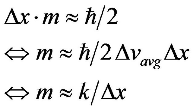
When measuring quantum mechanical properties an experimenter measures one quantum variable at the expense of randomizing a complementary variable. So there is in principle a certain amount of choice in where one takes one’s uncertainty. Using this thought as a guide, this paper makes another assumption, in order to simplify the mathematical approach. We assume that measurements are made such that there is a consistent distribution of uncertainties in velocity, which on average can be factored into a constant. In other words, measurements are made of position, and it’s complement momentum (velocity) is allowed to be randomized. We also assume that all measurements are made as well as possible, or at least with consistent accuracy, so that the inequality becomes an approximate equality. Using these assumptions, we can re-write Equation (1) as
 (2)
(2)
where k subsumes the constant and statistically averaged quantities. The author does not presume this formulation is the only possible one or that readers will easily accept it as an assumption. It is put forward as one method to make progress against a formidable problem, that of explaining the origin of inertia without resorting to the familiar but circular tools of momentum, force and energy.
Now consider the essential quality of mass. It is somewhere, in a particular state of motion, and the more massive it is, the harder it is to change its position or velocity. It is the opposite of our supposed mass-less or nearly mass-less entity that is “everywhere”.
If we add together many small-mass but vaguely-positioned entities, we do not get a larger entity with the same superposition of position states. The wave function becomes more concentrated and localized about a position and trajectory, which except in certain exotic experiments becomes easy to visualize and consistently measurable. The entity when so summed becomes a “particle”, and at macro scales, an “object” with extremely definite position. The addition is non-linear with respect to the concentration of position.
Consider now the introduction of a particle into the universe, one which ultimately will not be mass-less, but which under our assumptions will not have inertia until there is some kind of interaction with the other masses of the universe, or with fields or space-time metrics associated with them. One may consider this only a thought experiment, or one may consider it a real description of what happens when a particle is produced, for example by decay of other particles or of a photon. Even if the inertia is inherited, there presumably was an initial interaction at some remote time past in the creation of the universe.
Initially, before it acquires inertia, this newly minted particle will be as indefinitely positioned as our massless entity, existing in a superposition of states of being everywhere and at every velocity. It is capable of interacting with any other object-particle-field in the universe immediately, without delay. We know from quantum theory and careful quantum measurement experiments that though the particle may not use this property to “communicate” information between remote regions, it in fact does affect the state function of the particle everywhere whenever there is an interaction anywhere.
These quasi-measurement interactions are measurement-like. They are not carried out by 3rd party observers and do not result in complete collapse of the particle’s wave function. But apparently they result in its partial collapse, so that for more massive particles, the wave function becomes more concentrated about a position.
The particle’s state function gets information about the distribution of other matter in the universe two ways. At locations where it can or does interact (we cannot tell exactly whether it potentially or actually interacts, because we do not see these interactions, at least not in a form we recognize), then its state function logically would be updated to reflect something about the location of the other mass with which it interacted. The more frequent or intense such interactions would update the state function to reflect greater proximity. At locations where it does not or cannot interact, the entity gets negative information, that there is no matter present there, and its state function is not constricted by the regions devoid of matter.
The reader will have noticed the solution to many long standing puzzles in this simple qualitative argument. Since Newton, scientists have been resistant to the notion of action-at-a-distance. But the mechanism of quantum measurement and wave collapse is exactly such a mechanism, verified by many careful experiments. On the other hand, quantum measurement meticulously avoids communicating anything faster than the speed of light, and does not in any way violate special relativity. But the wave collapses instantaneously.
In the next section we will show how to quantify the production of inertia from the quasi-measurement interactions.
3. Derivation of Potential
Gravitational potential energy has historically been viewed as a fact owing to the ability to extract energy from falling objects. In the case of a single object M, the potential at radius R is
 (3)
(3)
Summarizing the historical approach, as an object m approaches M from infinity in free fall, it gains a positive kinetic energy –mVM and the system develops a negative potential energy mVM so that the total energy change is zero, less any energy that is radiated. Potential can be generalized for multiple masses by a summation, and further generalized for the case of masses in various states of motion by the use of field equations, such as linearized GR [9], giving a generalized gravitational potential VG.
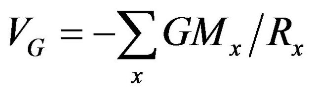 (4)
(4)
Continuing to summarize the historical view, in previously mentioned discussions [3-7], inertial mass was taken to be a function of, or approximate proportionality to, generalized gravitational potential.
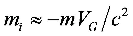 (5)
(5)
For objects in space not near any large gravitating body, it is assumed , and indeed astronomical observations bear this out to within the limits of observational accuracy [10].
There have been three philosophical objections to formula .
One is that inertial mass would seem to be not always identical to gravitational mass. Or if it is, and  is not exactly equal to 1, then the mass of the universe is unstable. In the author’s opinion, this is a reference frame problem. The mass-less entities supposed as the initial state of particles would have some weighting factor in the quasi-measurement interactions which produce inertia, which is unknowable since we cannot make measurements in that mass-less initial state. But we can make mass measurements of real particles in an arbitrary reference frame and use those as the proto-masses m on the right side of .
Another interesting objection, although not universally held, is that should be a vector equation, and inertia should be anisotropic near large masses. Recently a proof has been given using the Equivalence Principle that inertia based on potential, whether in a region of gravity or acceleration, has no directional component [11]. Apparently, inertia is not produced by a vector-type interaction between masses, and is not, for example, analogous to counter-motive induction forces in an electric field. This observation suggests that inertia arises from a density of interactions which is locally without a vector component. It might have a gradient, but isotropy experiments confined to a sufficiently small area could differentiate a gradient from a vector component. So we refine our assumption regarding the generation of inertia, and assert that it arises from a density of quasi-measurement interaction, which is without explicit vector qualities and is local to the position states the particle obtains after inertia is generated, governed by the uncertainty principle.
The final objection to (5) is that it is based only on classical physics, and has neither quantum rationale nor relativistic compatibility. To the relativistic quantum physicist, it at least conceals a deeper truth.
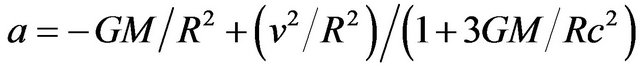
Using (3), we put (5) into the form of the inertia generated by just one other entity, using VM relative to that entity, with the understanding the observable rest mass in remote space M or m is only a proxy for a pre-inertial mass generating capacity. Substituting for VM we have
 (6)
(6)
If the radius R is taken to be the quantum interval Δx, that is, if we look at the position-momentum states in which the two entities might be directly interacting, because the uncertainty of their position is of the order of the separation between them, then we can substitute x for R and now we have
 (7)
(7)
Now we have the same form as the last version of (2), the uncertainty principle. Though it begins with classical constants instead of quantum ones, it makes the same statement as our assumption that inertia was generated by quasi-measurement interactions governed by uncertainty. The advantage of the quantum statement is that it does not contain classical values which ambiguously depend on inertia: m, M and c. The advantage of the classical statement is that we can measure all the values in it.
Both (7) and (2) should involve summations to obtain the total mass of a particle as contributed by all masses in the universe, and in the case of (2) also a sum of the interactions with all components of an aggregate mass M. We do not have enough information at this time to specify whether all interactions are of the same or different intensities or what their size is, so it is sufficient at this point just to “count” hypothetical same-size interactions in determining mass. Thus the law of conservation of energy, which we take as an assumption, reduces to maintaining a constant count of the total number of interactions.
While the classical view was that force diminishing geometrically as 1/R2 was fundamental, and 1/R potential a consequence of integrating to obtain energy, the view here is that 1/R potential from uncertainty is fundamental. We claim this only for the mass-causing field of quasimeasurement interactions, not for any other kind of field. The uncertainty based interactions decrease linearly rather than geometrically because they are independent in each orthogonal direction, rather than space filling. This gives rise to the well known property of potential-based inertia that equal thickness shells of mass at great distances are more influential than those nearby [5].
The remainder of this paper will show how resistance to acceleration and a convincing form of relativistic gravity emerge from such an inertia formulation. We begin by reviewing the transformations of mass, time, velocity, force and acceleration when measured across a difference of potential.
4. Laws of Inertia
Combining and we can write the inertia of a mass m as a direct summation of the contribution factor from each other mass, bypassing the abstraction of potential:
 (8)
(8)
As noted above, this summation is approximately “one” in normal space. In the vicinity of a gravitating object it is convenient to define an inertia factor, i.e. the factor of mass increase due to potential, as one plus the inertia due to the nearby mass [3,5]:
 (9)
(9)
The symbol Γ is adopted for the gravitational inertia factor, to distinguish from the Lorentz factor γ which increases inertial mass due to relative velocity. So in the above case . In a uniform field of strength g (acceleration) inertial mass is
 (10)
(10)
giving an inertia factor of
 (11)
(11)
The relative potential of any second reference frame as observed from a first reference frame is . If lowering a moving object (such as a clock mechanism) into a gravitational field, any velocity v must decrease by a factor of γ in order to conserve momentum, so we have
 (12)
(12)
 (13)
(13)
implying

where the primed quantities are measurements made in the original frame from which the clock is lowered, and the unprimed quantities are measured in the frame of the clock. No change is noticed in the frame of the clock. Since the ticking clock would appear slowed in proportion to v' then an observer remaining above the clock would observe fewer ticks, and more time between ticks, i.e. time dilation:
 (14)
(14)
If the object (still using a clock as an example) is not moving relativistically, then the Lorentz co-ordinate time transformation is not needed, only time dilation.
To complete the list of inertial transformations, we can easily derive that in order to maintain consistent laws of motion for all clocks, including electronic orbits, we must also transform acceleration and force:
 (15)
(15)
 (16)
(16)
It is not the actual force which changes, but its measurement, since the coordinates have changed. For example, consider a series of momentum impulses that would balance a force. The momentum of each impulse is conserved due to complementary transforms of m and v. But due to time dilation, the measured rate of arrival of impulses varies between frames.
None of the aforementioned laws change the shape of any trajectory or orbit (i.e. they cannot explain relativistic precession). This trajectory theorem is proved in [11], along with a more complete exposition of the above laws and their history. Only the force law was unknown prior to [11], but the acceleration law is not widely known.
Since the speed of light transforms as any other velocity (keeping in mind the locally measured quantities do not change, only cross frame measurements), light path delay is not alone sufficient to measure distances. We could reverse transform light path delays using the velocity transformation. Another practical possibility is to use orbits, which according to the trajectory theorem do not change size, only timing.
5. Resistance to Acceleration
We now consider the question of resistance to acceleration, as to why this should be related to mass, and what the essential notion of force is. Two arguments will be given, one based on momentum and one based on energy. The momentum argument will retain a conservation argument at its base, but will reduce that conservation to the preservation of an initial quasi-measured state. The energy argument will likewise assume that energy (mass) is conserved, which we have above defined as a counting of quasi-measurement interactions, but will address the mechanics of this in regard to reference frames, extending our argument that there is no preferred reference frame in the case of relativistic motion.
What is motion? In the first place, it is always motion of something else. The mass m never is moving in its own reference frame. Its state function remains centered about its position. But in another reference frame, the future state functions of m may appear progressively shifted in position, and that is what we call velocity. The fundamental relationship of the quasi-interactions which defined the narrowed state function of m, and its mass, is changing. It is easy to imagine that this is simply impossible, and that is exactly the position we take-in the aggregate. No object can move itself. It is fixed forever in relation to the other masses.
We introduce the assumption of single (or static) measurement. According to this principle, any particular isolated partition of matter and energy is measured but once, and whatever position and velocity it is granted by this process remains forever unalterable. In the reference frame of the center of mass of the partition, velocity is always zero. An ordinary centroid computation, weighted with mass and distance, then corresponds to the known macroscopic law of conservation of momentum. If the component masses of m are mj and their future distances from the original position are ∆xj, then .
.
From this, conservation of momentum  easily follows.
There are two escapes from this principle, which are well known from the classical law of conservation of momentum. By the rocket principle (action-reaction), energy or material may be ejected from a partition (group) with a corresponding reaction of the group. In this case, the velocity of the center of mass of the group is still zero, though the shape of the group distorts radically.
By the interaction principle, any part of one group may interact either directly or through fields with any other group. In this case, a new partition is drawn around the interaction parts, and the velocity of the center of mass of this new partition remains zero.
Whether this discussion adds any deeper understanding to the conservation of momentum is a question of philosophy. As far as physics is concerned, we have given the equivalent statement in terms of the quasimeasurement origin of mass and momentum, and it appears at least to be a reasonable assumption.
Force, then, must be a measure of the exchange of momentum. To obtain a concept of force, we use our earlier suggestion that a force is equivalent to a series of momentum impulses, such as for example:
 (17)
(17)
where  describes an arrival rate of momentum impulses completely absorbed by the mass m. Such a view is consistent with the position already taken by quantum mechanics that forces are transmitted through quantum fields by the production or absorption of virtual particles, i.e. bosons, the force carriers of the field.
For kinetic energy, i.e. inertial mass due to motion, the formulation is well known from SRT:
 (18)
(18)
where the factor γ is the Lorentz-Fitzgerald factor:
 (19)
(19)
and where c is the locally measured velocity of light, mi is the inertial mass of object m measured in the rest frame of m, and  is the inertial mass of m measured by an observer where each is moving with respect to the other at velocity v.
For our formulation of inertia to be consistent,  needs to be the result of an increased interaction density of the quasi-measurements. This cannot be due to Lorentz contraction of distances to distant masses because direct use of source masses might attach the effect to a particular reference frame defined by the average motion of the distant masses.
In view of our assertion that the quasi-interactions do not convey information about relative velocity, only position, then a contraction of the interaction density by the factor γ in one dimension (along the velocity vector) produces exactly an interaction density contraction of γ.
Consider a mass m. It is by definition always at rest with respect to itself. No matter what its velocity relative to other masses, it always perceives that any change in its motion, say to give a velocity v' would cause it to perceive a higher density quasi-measurement interaction field, and thus to experience more interactions.
By our postulate of conservation of energy, these interactions cannot simply be manufactured. They have to come from somewhere. If the existing mass m represents a certain interaction density, then the increase is given by .
.
Consider the case where a mass m is moving at near the speed of light, and a force is applied which, in the lab reference frame, would slow m down, thus reducing its relativistic mass in the lab frame. The energy removed from m is transferred to something else in the lab, and this case is not difficult.
Now consider the same case from the original reference frame of m. In that frame, before the acceleration, it appears that the quasi-measurement interaction density perceived by m would increase, so m will not oblige to change its state of motion without the necessary energy. In the old pre-acceleration frame of m, if we imagine some observer to be continuing in that frame, the mass of m has indeed increased.
The mass of m in its own present frame, of course, never changes as we pointed out earlier, because of the compensating effect of time dilation. But the mass of the lab has significantly decreased. The external mass (energy) of the universe is not conserved across an acceleration event in the frame of the accelerated object.
To clarify this position, consider a hypothetical case in which there existed an absolute reference frame. In that case, one might suppose that quasi-measurement interactions were absolute events, and only the mass of objects moving relative to the absolute reference frame would have increased mass according to the Lorentz formula. Then to reduce velocity would release energy, not require it, and might be expected to happen spontaneously, just as electronic orbits of high energy decay spontaneously to lower states, with the emission of photons. So far as we know, this does not happen, and energy is instead a quantity which exists relative to a reference frame. By contrast, momentum is conserved across reference frames.
It is well known that Newton’s law of motion  is equivalent to the laws of conservation of energy and momentum, and either can be derived from the other. The new elements in our discussion are the mapping of the conservation laws onto a quantum model of inertia causation, one which is independent of the reference frame of the source masses, and the demonstration that inertia caused by mass proximity and inertia from relativistic motion have a consistent explanation.
6. An Imbalance of Uncertainty
We will now deal with gradients in the quasi-measurement interaction density. Suppose a particle m moves lower in a potential field so that
 .
.
Because of the larger mass term , the product
  can be smaller than
  while still upholding the uncertainty principle. What this means is that as the object goes lower in the field, either the uncertainty of its position or its velocity or both will decrease.
Consider the mass m in Figure 1 shown at two positions, with two values of inertial mass mi and . Let the dashed circle represent the space in which there is some fixed probability ϕ of finding m (e.g. in a particular measurement). The probability of finding the particle outside the circle is
 . If ϕ is chosen to be near to 1, i.e. to include the area in which the particle will most likely be found, then
  will be very small. Because of the increased mass at the lower position, the area for the same probability ϕ is smaller.
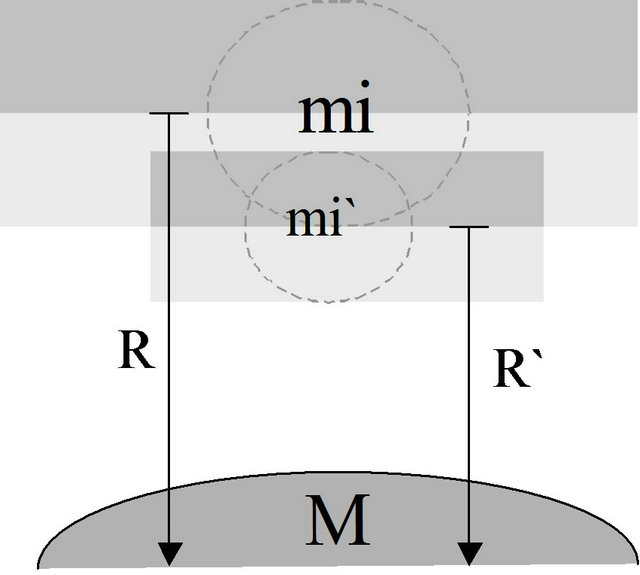
Figure 1. Imbalance of uncertainty.
The probability described here is related to the particle’s wave function. The wave function describes the probability of finding the particle as a function of space and time. Time is dilated for a particle at , so the wave function is stretched in time as perceived by an observer at R. The particle does not perceive its probabilities changing any more than it perceives its mass changing. But to an observer at R, the probability of a particle at R later being observed at
  within a fixed period of time ∆t, is greater than the probability of the particle again being observed at R after having been observed at
 , also within a period ∆t, where ∆t is always measured at R.
The main concern is with the probability of finding the particle higher or lower, not with horizontal motion. The expected value (or average value) of the position of the particle is at its current location. Divide the space about the particle into two regions, above and below the current position, shown by the shaded bands. Let the upper edge of the dark band represent the expected excursion considering only upward excursions, and the lower edge of the light band represent the expected excursion below the current position, within some interval ∆t. By excursion, we only mean the probability of finding the particle in a measurement. The particle need not actually move. It exists in a superposition of states, and we call a measurement an “excursion” if the particle is not at the nominal (last measured) position.
There is an imbalance of probabilities between the positions of mi and  due to the difference in inertia between mi and
 . The lower position is illustrated to be at the expected excursion from the upper. But once down to
 , the expected upward excursion is less than what is required to return to R.
An hypothesis is put forward that if there is an interaction that causes the probability envelope of a particle to change in both size and position, then motion is induced. This interaction need not be an explicit macroscopic measurement. It may occur in the quasi-measurement background interactions.
For example, if for a particle nominally at R there is an interaction at , allowed by the uncertainty principle, which causes the particle’s probability envelope to be constricted based on location at
 , then the particle’s position would have shifted. It seems that the object would more likely be found at the lower position after some time. Not only would its position have changed, but it would acquire some velocity, based on the time interval and the distance between observations. Once created, the velocity would continue due to conservation of momentum. (Of course, the position and velocity of a companion large object M causing the gradient will also shift, conserving momentum.) After a further time interval, the object would likely relocate downward again. As reasonable as this argument seems, there appears to be no precedent for it and no established way to calculate such acceleration.
Note that the particle m does not “move” from R to . It is discovered by a measurement-like interaction at R, and some ∆t later it is discovered at
 . In between, it existed only as a superposition of states. Experiments involving entangled particles and the Bell theorem suggest that it is pointless to think of it existing as a particle in between. While this does not make hidden variable theories impossible, it does require them to embrace superluminal communication, which for the purposes of this paper can be bent to the same end result as far as the behavior of particles in a potential gradient is concerned. In either case, processes inside the wave packet are not limited to the speed of light.
7. Imbalance Becomes Acceleration
A few minutes spent considering alternatives for calculating the acceleration due to the change in uncertainty in a potential gradient reveal that there is a missing parameter. There are relations which provide a maximum bound of momentum and position, or of energy and time. There is not a relation that says how quickly, at maximum, these values can be updated. This becomes a free parameter.
In order to quantify the free parameter, we will use hypothetical opportunities of measurement at various points. We will imply that these form a sequence in time, and as in the above discussion, any pair in the sequence will imply a velocity, even though there is not any physical particle moving between the points, only the superposition of states allowing discovery at either or both of the points, according to the probabilities of the wave function. It is only a model for computation of a quasi-interaction update parameter, not a description of a physical process. Further take any changes in uncertainty as being applied to ∆x, for convenience in calculation, based on the same rationale by which we already chose ∆x for the inertia derivation. We do not assume that the opportunities of discovery are identical to the quasimeasurement interactions. They may be, or it may be that many quasi-measurement interactions are necessary to update a particle’s mass. The opportunities for discovery are only assumed to be points at which the particle’s mass can be updated.
Figure 2 shows conceptual drawings of how the opportunities for discovery might behave in purely computational model. The opportunities for discovery are the vertices of the line graph, and the line shows ordering, not path of motion because the particle may exist only as superposed states between discoveries.
In Figure 2 part (a) there is a random gyration. This is not of much use. In part (b) we show a gyration to the side and back. Side and back gyrations of equal length occur with equal probabilities, as no change in mass is involved, and can be ignored. In part (c) we show gyrations down and up, which do not occur with both equal probabilities and expected values.
In the following model an update of mass is supposed at the end of each excursion (out is one excursion, back is another) which causes the probability envelope to be re-determined. In the vertical direction this gives unequal excursions, –h and +h/Γ, where Γ is the relative inertia factor . Examining only the vertical components of excursions, since the horizontal components don’t create acceleration, this can be diagrammed as in part (c).
If one could discover how rapidly the process in Figure 2 part (c) repeats, one would know the acceleration attributable to the potential gradient. However, this appears to be a free parameter, so instead the converse procedure will be applied. Assuming that all the acceleration g manifests through this mechanism, the free parameter will be determined.
8. A Hypothetical Velocity
Several factors are apparent. How many of the excursions are vertical? How often do the excursions happen? With an observable particle like a large molecule, we would eventually determine all these parameters. Inside the hidden quantum world it is not a very useful approach. Instead, one can make quite arbitrary assumptions about some of these virtual quantities, and let the remaining quantity be the free parameter.
Consider again only excursions of the out and back type, with equal probabilities in equal time periods, and only their vertical components. Given two points and a time interval (in this case, the points of update of mass, or points of discovery), we impute a velocity, even
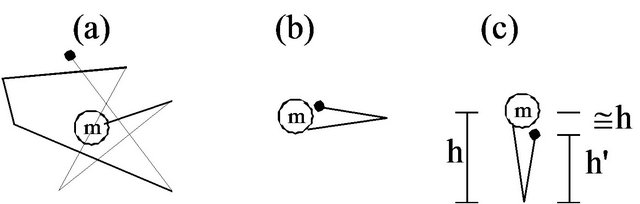
Figure 2. Hypothetical point of discovery configurations.
though nothing observable is happening between the two points and no path or continuity is implied. This “velocity” will only be used as a proxy for computing time intervals. Assume that the vertical such velocity component is always , meaning “effective” or “equivalent” velocity. Assume that as soon as one out and back excursion ends another begins. The author cannot emphasize enough that we are not postulating a physical process. We are reducing an unobservable physical process to arbitrary equivalent elements. It is a computational model, not a physical model.
Let all measurements including time be made at the original particle position, so that for the two excursions . One can now solve for acceleration by first finding ∆h. We have
 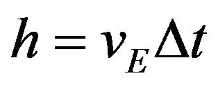 and
and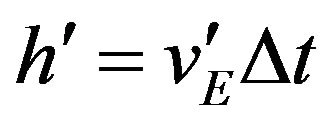 . We have
  from (12), giving:
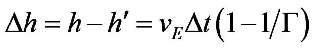
Since  is very close to 1 for small h, we use the approximation that for
 ,
,  , giving:

An expression can now be written for the velocity v imparted to the particle m over the interval of the entire excursion pair 2∆t. This will yield the average velocity  over that interval. Assume that the velocity at the end of the interval will be double the average velocity.
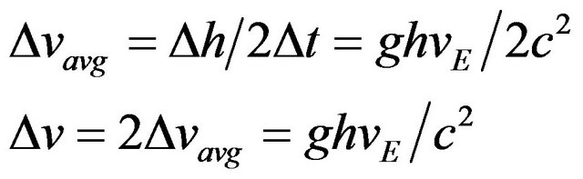
Now solving for the acceleration a:

and substituting for h:
 (20)
(20)
It turns out that the height h of the excursion does not matter. It cancels out of the equations. So does the time period ∆t within which each half of the excursion takes place. With the restrictive assumptions above, that leaves only . This one parameter rolls up all the other various parameters. The free parameter can now be chosen as
  giving
 .
.
If the sequence of mass discovery points is described by continuous vertical excursions at the “equivalent” superluminal velocity , then gravitational acceleration along a potential gradient can be viewed as the influence of inertia on the uncertainty of the particle’s position.
Notice that the particle’s mass, either gravitational or inertial, was not needed to deduce the acceleration, just as one would expect from the Equivalence Principle. The acceleration appears directly. If a force is applied to resist the acceleration, this must be proportional to the particle’s inertial mass.
This view of gravity does not stray from the basic premise that forces are conveyed by interactions with a virtual particle field. Acceleration arises from the influence of the inertia-causing field (of quasi-measurement interactions) on uncertainty, and a force must be applied if one resists acceleration, which corresponds to the intuition of the free falling observer as Einstein suggested.
One further thing is interesting about this hypothetical velocity . Computing the Lorentz factor
 gives
gives . So length and time aren’t contracted or dilated and mass isn’t increased, but all these quantities are imaginary, if the Lorentz factor has any meaning in this situation. In other areas of physics and engineering,
  often signifies real behavior, but of a different sort than expected. Quantities which are conserved under Lorentz transformation, like the real momentum of the particle, would still be real, and still conserved. Presumably the particle remembers its momentum, even when unobserved, as well as its charge and gravitational mass, and the sequence of opportunities for discovery must conform to the conservation of momentum, even while by virtue of the quantum veil it is exempt from other velocity restrictions.
9. Orbital Predictions
Note that in (20) acceleration depends on the ratio . VE and c both depend on Γ via the velocity transformation (12) which is necessitated by time dilation. The Γ factors cancel, and thus from any particular point of view, acceleration itself is not a function of relativistic parameters, and to a fixed observer appears undiminished by relativistic effects. We will now show that this condition leads to orbital precession values in close agreement with General Relativity.
For a comparison baseline of gravitational effects the Schwarzschild metric will be used, which is known to give a correct result for planetary orbits in the solar system. Taking the form given by Brown [12]:
 (21)
(21)
and re-writing using our notation and units, we have
 (22)
(22)
For  we can use the small x approximation,
  , thus:
 (23)
(23)
Since is in the frame of the object, which is free falling, a = 0. What we have left is the balance of gravitational acceleration and centripetal acceleration. The Newtonian centripetal acceleration is reduced by  which can be factored, ignoring high order terms, as
 , where
 .
.
We can rewrite (23) as
 (24)
(24)
Whenever equations of orbital motion in the frame of the orbiting object can be reduced to this form, the observed value of planetary precession will be obtained.
We can derive a relation between the gravitational relativistic factor for weak fields, Γ, and the lateral velocity Lorentz factor . For circular orbitstangential velocity is given by:
 (25)
(25)
This is a good approximation to average velocity for near circular planetary ellipses if R is taken as the semi major axis. Substituting for v in the Lorentz factor formula and using the usual approximations for operations on 1 ± x for  we have:
 (26)
(26)
The total relativistic transformation factor for an orbiting mass will then be
 (27)
(27)
Figure 3 shows how an accelerated frame of differential width ∆x can be applied to an orbit. For simplicity, a
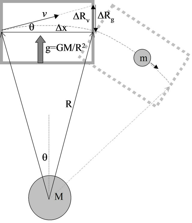
Figure 3. Orbit represented with accelerated frames.
circular orbit is assumed, which allows the orbiting object to enter and leave local accelerated frames conveniently at the same height R. In the limit as ∆x → 0 an accurate representation will be obtained.
Setting the radial displacement due to gravity ∆Rg equal to the radial displacement outward ∆Rv due to inertial continuation of v gives the expected result for balanced gravitational and centripetal force,
 .
.
This equation has been derived so far without regard to relativistic factors. Accounting for m’s relativistic motion, notice that centripetal acceleration v2/R doesn’t change. A new ∆x is marked using m’s coordinates, leaving the diagram of the accelerated frame unchanged. The number of ∆x’s that m finds in an orbit is not a factor since neither R nor v changes. However, the constant gravitational acceleration will be perceived through m’s time dilation and must be transformed by the inverse of (15) giving:
 (28)
(28)
This has exactly the same form as our benchmark (24).
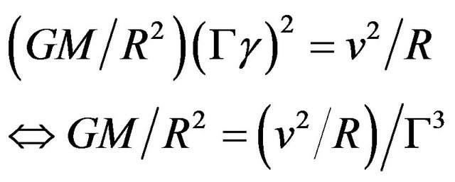
This shows the precession agrees with experiment. But how does an observer at m understand the additional acceleration and write equations of motion? It is apparent that certain physical constants used in connection with quantities that are transformed by inertia may themselves require transformation, and the gravitational constant G is one of those. In order to make acceleration constant in the remote reference frame, then the gravitational constant must be transformed like acceleration, and we have a new law of inertia:

Note that when written according to the conventions of the other inertial transforms, the primed frame is the remote observer. But in the orbital analysis  corresponds to our normal gravitational constant.
The reader may wonder if we can and should use Γγ in all the inertial transformation laws. Whenever the quantity transformed is scalar (such as time, above), or a vector at right angles to the relative motion, there is no difficulty in this. But for components parallel to motion, we run into the Lorentz length contraction, and the Lorentz transformation of time as a function of displacement along the direction of motion which de-synchronizes clocks (time skew) in one of the reference frames.
In the case of transformations of components along the direction of motion, the full Lorentz transformation may be viewed as composed of two parts. The first part is just the transformation indicated by the laws of inertia. The second part is the length contraction, which must also be associated with time skew.
10. Light Paths
Time dilation, and the consequent velocity slowing, will have a steering effect separate from any falling effect. Referring to Figure 4, consider two parts of a wave or particle separated by ∆h and traveling horizontally at v and v2 respectively.
After a horizontal interval ∆x we have , and we assume
 . Two formerly vertical points on the object will be turned at an angle ϕ such that
 . The velocity vector v will be turned by this same angle ϕ so that a vertical velocity component ∆vh is added, where
 . Equating the two expressions for ϕ we have
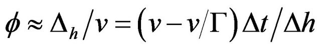 . We can rearrange this into an expression
 . This value ∆vh/∆t is aligned with the gravitational acceleration g (assumed to be vertical in the figure). Substituting for ϕ using , using for
 , and simplifying we have:
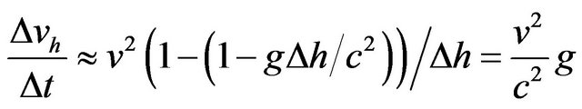
For light, we have  and therefore
 . Since
  is added to the explicit acceleration g as already noted, we have a total apparent acceleration of 2g. This value is well known to agree with observations of stellar deflection in the vicinity of the sun [13,14].
11. General Laws of Motion
Two body problems. Consider two masses A and B, a negligible test mass X in between them, as in Figure 5.

Figure 4. Setup for speed gradient refraction.
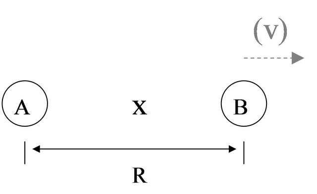
Figure 5. Two body problem with test mass.
The test mass x derives its inertia from the two masses A and B, . It matters not whether there is any relative constant motion v of A or B or both, by our hypotheses. At the instant of the configuration of the figure, the defined distance from x to either mass is
 .
.
Take this configuration as our baseline reference, and now consider what happens if R is doubled. The inertia at x is half. An observer at x still measures c at 3 × 10⁸ m/s, but any object that had started moving during the old conditions of smaller R will now be going twice as fast in reference to the original reference frame, including photons. But its measured speed, by clocks ticking twice as fast, will be the same, and its transit time will be the same. The fact of a doubling of all distances in this “universe” will be un-noticeable except for a halving of the wavelength of any old light emitted before the expansion. Thus inertia theory implies a certain relativity of distance.
We note that the stretching of the wavelength of light in this instance is remarkably like the stretching of light in the case of space-time expansion in metrical theories, and is calculated the same way. This is in addition to any Doppler shift due to underlying relative velocities separate from the expansion.
Notice that regardless of the value of the proto-masses mA and mB, the inertial mass of each of A and B is proportional to the product of the two proto-masses, so that  always in a two body system.
We now modify our thought experiment in a manner that is not possible, even in theory, but which serves to illustrate the interconnectedness and relativity of inertial relationships. Assume that . Suppose that suddenly B were given an outward radial velocity v as shown in the shaded part of Figure 5, while A were held in place. X’s distance had been defined equally with respect to A and B. Now one of them accelerates away. If x were very close to B and its inertia almost entirely defined by B, then it would accelerate away with B, remaining in B’s reference frame, and vice versa if it were close to A. Given its position half way in between, it will accelerate away at half the rate of B, maintaining but scaling the original relationships. X would feel no force, and its path of motion would be analogous to what is called a geodesic in metrical theories. It would be impossible to tell whether A or B had accelerated, or both.
Frame dragging. We have treated inertia as an aggregate result of summation, making an exception only for proximity to a single massive object with the “one plus” formulation of (9). This is valid in the case of a more or less homogeneous universe, but not in the general case of cosmological situations, or even of multi-body massive object situations. In [11] it is found that the laws of inertia coincide generally with GRT in describing gravitationally captured objects, in which most of the inertia of an object is due to a massive proximate neighbor. It is very difficult to move the smaller object relative to its position in regard to the massive one. But this is only due to the inertia of the small object relative to the massive one. Inertia is not absolute. The two objects together may be moved with the same total effort as they could be before they were brought close together, for their aggregate inertia relative to the rest of the universe has not changed. Similarly, in GRT, near the horizon of a black hole, it is basically impossible to move an object due to time dilation. But the entire black hole can be moved. The mass of the black hole plus the in falling object is no greater than the sum of the two when separate.
In [11] inertia was found to be isotropic. This means it is as difficult to move the fallen object tangentially as it is radially. If one then starts a rotation of the massive object, the in fallen object will be dragged along in the same relative position just as x was dragged in the two body example above, and this phenomenon is analogous to frame dragging in GRT. However, if a falling object gradually comes into proximity to an already rotating object, it is less clear what happens. Acceleration causes dragging, but the acceleration of uniform rotation is not tangential.
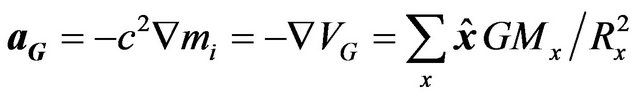
A vector co-variant acceleration field. In the frame of a distant observer at normal potential (Γ = 1) and applying only to non-relativistic objects (slow moving, not in deep gravitational fields) we can formulate the law of gravitation based on linear decomposition
 (31)
(31)
where  is a unit vector from m to Mx, and which for a single “other” mass M reduces to the classical law as it should in the non-relativistic case
 . The mass of the falling object m or mi does not enter the equation, upholding equivalence. For rapidly moving objects or deep gravitational fields, other factors are needed, but first we’ll develop a simple co-variant equation of motion.
In order to be able to sum the gravitational acceleration with actual forces acting on an object to obtain its net motion, we can obtain a pseudo force version of (31) by multiplying by mi, the effective inertial mass.
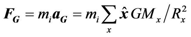 (32)
(32)
The second rule is frame dragging from any accelerations of the masses Mx. These are attenuated according to the proportion of the inertia mi due to object Mx: 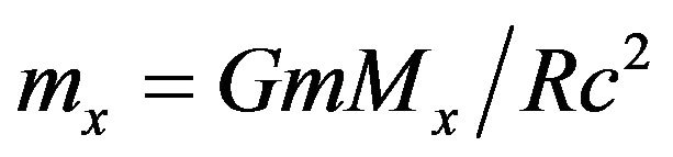 giving:
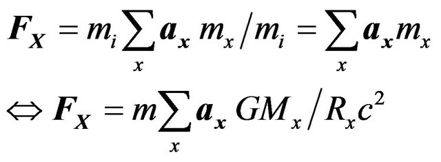 (33)
(33)
After a moment, one realizes that (33) is a re-statement of Newton’s law of motion, without using inertia. If an object has acceleration a due to an applied force, then in its frame all the Mx appear to have an incremental acceleration −a, which produces a frame dragging force −F that exactly balances the applied force. The constant acceleration −a can be factored from the summation, and the remaining summation is recognized as the inertial mass mi, and the equation reduces to , the mirror image Newton’s law of motion, giving the force of inertial resistance to acceleration.
It would appear that it is a simplification to think of inertia as being due to a scalar potential defined by a quasi-measurement field. This simplification is useful in calculating local motion, such as the rate of clocks. But in fact inertia appears to be only a special case of frame dragging. Taking the general notion from [11] that time dilation implies inertia increase, and observing that GRT already has a notion of frame dragging, one might conclude that if not already contained in the usual metrical analysis of GRT, something like Equation (33) should be added. This finding that inertia is a special case of frame dragging would appear to apply to a large class of theories.
In addition to the unexpected link between inertia and frame dragging, it appears that the sum of aG and aX (or pseudo forces FG and FX) is zero in any reference frame, such as that of a free falling object. Therefore, in an arbitrarily moving reference frame, for an object m, the sum of all accelerations is zero (free fall) unless there is an applied force, FA, so we have the following co-variant law of motion:

In a strict 2-body problem, there is no way for the bodies to apply force on each other, outside of gravitation. Any energy exchange between them would constitute additional mass not localized at one of the two bodies. Notice that since each object gets all of its inertia from the other in a 2-body problem, that whenever one object experiences an acceleration from the gravitation of the other aG, it imparts an equal acceleration aX to the other due to frame dragging. Therefore, a strict 2-body system would continue its initial velocity indefinitely.
Angular momentum. It would be remiss to offer a theory of inertia without discussing it in light of the famous thought experiment given by Newton, in which a bucket of water is rotated in an otherwise empty universe, and the water nonetheless crawls up the side of the bucket as normal. Ernst Mach disputed this claim, and countered that if the universe rotated about the bucket, the water would react as if the bucket were spinning. Brans gives a summary of the debate in the context of current theory and recent experiments [15].
Equation (34) can be used to define angular momentum in the usual way, where two or more masses are bound, causing linear momentum to become a rotation in the presence of a centripetal binding force. The binding force acts perpendicularly to the rotation, and other matter in the universe is perceived as countering with outward radial acceleration. However, the direction is different at every point in the rotation, so that the symmetry necessary to support Mach’s argument does not exist. The acceleration vectors of a rotating universe add up approximately to zero. The author is preparing a separate account of this unexpected result with illustrations.
12. Relativistic Motion
The purpose of this section is to formulate the simplest possible equation to use for investigating how quasimeasurement field dynamics might affect cosmological situations in which velocities are highly relativistic.
Speed of propagation. We have based inertia and gravity on a quantum measurement process which does not violate SRT even though correlated measurements appear to be instantaneous in some frames, or out of order in others. But our intuition may not be comfortable with this idea, because it seems as though we could “wave a mass around” and generate a signal at some remote location. There is a tendency, even on the part of the author, to think that surely changes in the quasi-measurement field must be limited in propagation speed. So this discussion section will address this disconnect between our strong intuition, and what has been derived and observed.
A “signal” would be a gravitational wave. Physicists have been looking for such signals for many decades, with large expensive experiments that were thought to be capable of finding such signals. So far at least, none have been found.
The Newtonian limit of gravitation is well known to only give correct results if one assumes un-delayed signals. GRT as a superset also has this property. How GRT accomplishes this is not at issue here, only that it does, and this mystifies non-specialists and even many graduate students. Our theory is no different than GRT in this regard.
Since gravitation and inertia are universal, one cannot “wave a mass around” without waving the waver as well, so that the center of mass does not move and only near field signals can be generated. These local signals require propagation of the masses themselves, which is limited by SRT. Consider a stellar explosion. It will be roughly spherical, and until one comes within the outer layers of the expanding sphere, the gravitational field is unchanged.
A second difficulty also arises because of the universal action of gravity (and frame dragging). It affects everything. So how does one detect a signal? This is closely related to the Equivalence Principle. One cannot determine the difference between being in a gravitational field and being free of gravitational effects, except by looking for a reference beyond the suspected gravitational field. Suppose, then, something can hurl a mass from another planetary system into our vicinity so that we can detect its gravitational effects. To do so, we must rely on signals which propagate from outside the range of that effect after the mass is present. To minimize that detection delay, it will have to get close, which means it is traveling close to the speed of light, otherwise we would simply see it approaching.
Such an energetic event as we hypothesize cannot simply throw a pair of large masses in opposite directions. The energy release will be chaotic, tremendously increasing entropy, and thus going in every direction, producing the spherical case we already classified as undetectable.
If one postulates less energetic trajectory maneuvers, not only can we see them coming, most likely they can be predicted thousands of years in advance. If the event can be predicted, there is no communication. Since celestial objects are always mutually interacting, there is even an ambiguity about the ultimate cause of trajectory events.
Finally, if potential or gravity propagated as does an electric field, there should be a Lorentz force, corresponding to the derivation of magnetism from the electric field. The author’s own attempt to formulate inertia from gravitomagnetic induction did not produce a convincing result. Sciama’s somewhat different approach to inertia as induction [5] was criticized for appearing to require propagation backward in time, and Sciama never produced a promised second paper, though Davidson suggested the result was already contained within GRT [6].
How then do inertia events appear in different reference frames? In a particular formulation they may appear to have a different ordering, but as we have shown, this cannot have detectable consequences at remote locations faster than light travels. In other words, at a particular location, we cannot discern a detectable difference between using the equations of motion with state information brought to us on light rays, and the actual motions we observe. Some other observer, with a different light horizon, might observe our entire section of the universe being frame-dragged by remote events, but since everything including light gets dragged we have to wait for external signals to detect this.
The flip side of this is that we can use any information we do have to predict motion. For example, when an object accelerates, we can calculate inertia as if it is immediately interacting with the old positions of objects we see with old light, knowing there will be no perceptible difference to us, and certainly not waiting for induction fields to propagate from distant objects (as in the critique of Sciama’s theory).
Our conclusion is that having argued from the starting position of measurement type interactions which do not violate SRT, having found multiple blocks to the possibility of violating SRT in our final result, and having experimental data or lack thereof from gravity wave experiments and solar system dynamics, the burden of proof is reasonably met. If at some future time the gravity wave experiments are successful, and can be correlated with optical signals, then this aspect of the theory would need revision. Meanwhile, the peculiarities of measurement based interactions appear to offer unique solutions to historically difficult problems in inertia theory.
Limits of scope. By relativistic equations, we mean not only relativistic velocities, but also relativistic gravitational situations such as proximity to very massive objects. The full description of inertia theory for multiple proximate massive objects can be quite complex, effectively a set of N simultaneous equations with N variables in the case of N nearby massive objects. We will not describe this general case herein, although it may well be relevant and necessary for some astronomical and cosmological problems.
To give the reader a feel for the problem, consider just two very massive objects near enough that each gets a substantial portion of its inertia from the other. Their resistance to motion relative to each other can be much greater than the sum of their independent inertias, if each was alone at their proposed locations. But if we try to apply equations of motion independently to each of them using this large inertia, the result will be incorrect, because the pair together has no more resistance to joint motion than the sum of their independent inertias without the presence of the other, as we have previously emphasized.
In order to develop a simple computational model which is a reasonable approximation in at least some situations, we will exclude massive objects from having any nearby neighbors, unless a large group of neighbors are approximately equally near.
Equation for relativistic velocities. For our purpose we will use the reference frame of an observer at normal potential , even though in the cosmological case this is somewhat contrived. The reader may consider that we might as well assume some asymptotically small value of Γ which could be positioned at any remote vantage point, and we can use the laws of inertia to transform these observations into a
  reference frame. We do this not only to facilitate comparison with our natural observations, but more importantly, because the frame of co-moving observers, often used in GRT, does not seem to be available in quasi-measurement field dynamics.
To make a relativistic equation of motion we must account for factors which depend on the relative positions and velocities of the interacting particles. The transverse velocity in a gravitational field which produces double bending of light adds a factor of  to each gravitational acceleration term, where we use
  to indicate the transverse component of the velocity vector of relative motion between m and Mx. In the simple problems we’ll consider, primary velocities will be radial, and small tangential velocities that might arise among orthogonal directions will be balanced by symmetry, so we won’t use this factor.
We need a relativistic force law that references the rate of change of momentum, not velocity, otherwise violations of SRT would appear. But we do not have a force. The solution is to create the mathematical fiction of a “pseudo force” Fp by multiplying gravitational or inertial acceleration by the inertial mass of the falling object as measured by the observer:
 (35)
(35)
The mass mi is the full relativistic mass from both potential and relative velocity:
 (36)
(36)
where m is the rest mass of an object in the observer’s frame. We can now use the conventional formulation:
 (37)
(37)
where v is the vector velocity.
A relativistic equation of motion in a reference frame where  and where velocities and mass distributions are symmetric and velocities are radial can be found by substituting (37) into (34):
 (38)
(38)
Notice that if one wishes to handle particles traveling at the velocity of light, a wavelength formulation of momentum is needed to avoid an indeterminate Lorentz mass factor.
The FG term does not have an acceleration factor, but the FX (frame dragging) term does. In this case it is the acceleration of the remote mass MX. However, this is not an inertial mass, it is the pre-inertial mass generating factor (for which we have used rest mass as a proxy). As such, it does not have a relativistic form, and there is no protection from excessive speed from this term. But no protection is necessary since this term co-accelerates broad regions of masses.
13. Cosmology
The work of adapting GRT to cosmology occupied most of a century, and it is not realistic to adapt a new theory entirely in a single paper. But there is also an obligation address the feasibility thereof. We present here hypotheses as to how quantum inertial gravity might fit or explain various cosmological observations and theories, based on known properties of quantum inertia theory but without quantitative analysis as to sufficiency, which is left to future work.
Event horizons. Notice that since inertia and therefore the speed of light varies continuously across space, it is only meaningful to enforce SRT locally, just as in metrical theories. Objects at some distances from each other may have superluminal relative velocities. The speed of light is a local constant, but as viewed from other reference frames, is transformed based in the relative inertia just as any other velocity. Therefore, remote objects in a lower inertia potential can be moving much faster than the local speed of light. However, unlike GRT, it is not clear that there are any horizons at the cosmic level. Light propagating toward those distant objects would speed up as it moved through regions of lower potential (less inertia). Of course the propagation distance will be limited by the age of the universe.
Dense gravitation. The theory certainly allows massive, dense objects, which for any purpose outside the traditional radius of an event horizon resemble black holes. At ten times the gravitational radius, there is less than half a percent difference in time dilation, light paths, or other physics. At a mere 10% beyond the gravitational radius, there is still only a 50% difference in time dilation. Effects which occur at greater than this radius would be difficult to distinguish at interstellar distances. The mass at which neutron stars further collapse would be essentially identical. The endpoint of that collapse is an imponderable question in either theory.
Red shift. In an expanding field of masses, 1/R is constantly getting smaller as R’s get larger. This is a general case of the two body problem discussed above. To a neutral observer (e.g. at a great distance from the expanding field, or very near a massive object contributing most of the observer’s inertia), the inertia of the individual masses in the expanding field decreases with time. So clocks speed up, including photon emission processes. Therefore, observers in the field will have clocks that accelerate through time, and will view old light as red shifted, because it was emitted in a past epoch when time dilation was greater.
Expansion and accelerated expansion. Hubble-like expansion has been shown to be a normal, in many cases inevitable, endpoint of a system of masses in motion, with our without a Big Bang [16]. But inertia theory contains features that greatly encourage it. Consider the field of expanding masses described above. Momentum is conserved across reference frames with different inertial potentials. Therefore as the inertia of the masses decreases with expansion, their velocity increases to conserve momentum.
Figure 6 shows numerical solutions for six masses having a total of one solar mass, each pair positioned along one of three orthogonal axes of motion, initially at a radius of 1000 meters, given various initial velocities outward relative to the center of mass. The velocities are expressed as a percent of the local velocity of light. These masses are contained in our normal universe with a background inertia of . The chosen velocities are grouped about the escape velocity, approximately 70.7% of the velocity of light at this radius for this mass. The final trajectories above this velocity quickly become straight lines, indicating constant velocity, since the initial inertia factor is only about 2.5 times the background inertia.
Figure 7 shows the same mass configuration in an otherwise empty universe, with a background inertia of zero. In this case inertia continually decreases as the masses expand, and so there is a continual acceleration, shown by the concave upward trajectories, which persist indefinitely. One curve with double mass and double initial radius is shown also. Not shown are solutions for very low background inertias. Up to a background inertia of 0.009 the curves are similar to these, but when carried out far enough the acceleration ceases. At larger background inertias, the initial velocities must be substantially increased (like those in Figure 6) to avoid rapid collapse.
For the masses embedded in the normal universe, if analyzed by GRT or other metrical theories, these objects would be well within the gravitational radii of the group, beyond an event horizon, progressing to a singularity. In
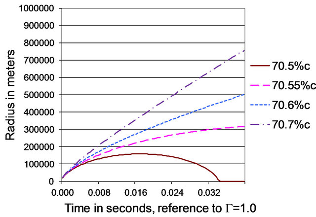
Figure 6. Six element solar mass expansion in normal space.
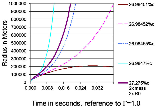
Figure 7. Six element solar mass cosmology.
quasi-measurement dynamics this is not the case. It is possible that two objects may part from any distance.
As a group of expanding masses pass beyond the point where their self-gravitation is the dominant force, and the acceleration due to decreasing inertia becomes dominant, then dark energy might not be needed to explain acceleration of expansion, or less of it might be needed. There seems to be potential for quasi-measurement inertia theory to fit cosmological accelerated expansion. Whether actual data fit using a realistic computational model will require extensive analysis and consideration of alternative configurations. Phase changes and all the attendant complexity of current cosmological models, with possible additional complexities, will be needed. It might be possible to determine if “other universes” exist by testing whether a small initial background inertia is required for models to fit astronomical data.
Isotropy. While the universe increasingly shows signs of large scale structures and flows as we observe it more closely, it is still usual to think of it as largely isotropic. This would be a difficulty for any flat space-time theory, were it not for other cosmological observations that indicate the universe is closely balanced so as to be nearly flat anyway. A field of expanding matter might appear quite isotropic from most locations. The asymmetry in velocities looking “outward” vs. “inward” might not be apparent, even over large scales, due to the inherent Hubble-like ordering and the possible dominance of aging red shift over velocity red shift. The greater time dilation looking “inward” would add to the apparent distance of objects in that direction. The increasing acceleration due to low inertia near any boundary would blur that boundary perhaps beyond recognition.
Dark matter. There is no practical difference between metrical and inertia theories with regard to galactic rotation curves. Dark matter is still required.
Inflation. Looking at an initial small dense universe, the reverse of arguments regarding acceleration of expansion can be made. Suppose the initial expansion, caused by whatever caused the “Big Bang” (which is not addressed by any gravitation theory), was highly superluminal. It is not clear that such a state is prevented by SRT, since the relative positions of masses may not be changing very fast, if at all, and no local violations of SRT may be observed. Time dilation would be severe because of the density, and inflation would occur in a very small amount of time relative to an embedded observer. In this case, either the self-gravitation or other energy phase change process, along with diminishing time dilation, contributes to the end of inflation. The author concedes that much more work would need to be done on this conjecture, but feels it likely that some of the work already done could be adapted.
Special Relativity. The variability of the speed of light in inertia theory provides no relief for space travelers or communicators. Consider the geometry of potential. The fastest potential can diminish and speed increase is 1/R. But any path between objects, owing to geometry, would increase at least proportional to R. Adding the time required to ascend and descend in the potential field, it seems likely that a proof could be given that it is not possible to find a better path between objects than that of an ordinary light ray. Indeed, inertia theory, with its complete agreement with established theory on light bending, is compatible with the path of light as a minimum time path.
Multi-verse, brane, and string theories. Quantum-inertia theory does not say anything about higher dimensions, neither requiring them nor ruling them out. It does offer a kind of alternative to the multi-verse theory, in which there might be very large accumulations of matter (universes) with vast separation between them. This would preserve the fractal structure we have seen so far in observations of the cosmos. It might not be completely impossible to travel between such regions. The inertia field would be very low in the void. Little time would pass in the dense material regions while a traveler was moving between them near a speed of light which is much greater than the speed of light in the dense regions. But the traveler’s clock, correspondingly, would be ticking very fast, perhaps even after relativistic time dilation is considered, so some means of preservation would be required. As in other relativistic travel scenarios, the universe of origin would likely be gone before the traveler could return.
14. Verification
There seem to be three important verification questions (at least). First and most important, a new method of producing equivalence is described. The existence of this method suggests that demonstrations of equivalence do not exclusively confirm metric gravity. Even if the method is ultimately found to contain some flaw, it suggests a direction in which one can look for additional methods of producing equivalence. Since equivalence is a pillar of the verification of General Relativity, a new verification issue arises with the metric theories [1].
Second, while use of a classical 1/R potential function, as supported by our argument deriving it from the uncertainty principle, gives agreement for planetary orbits in the solar system, orbits near the gravitational radius of an object would differ. Seeing no obvious reason to deviate from our 1/R arguments, we tentatively suggest that direct observation of light bending or orbits in the vicinity of what should be the gravitational radius of a massive object, would allow differentiation of our theory from metrical theories which predict an event horizon. But if the gravitational radius is obscured, or if attempting measurements within the solar system, we will find some difficulty owing to the close agreement. At one million times the gravitational radius (about 2 million miles in the case of the sun), predictions of time dilation differ only in the 13th decimal place.
Third, experiments need to be suggested and formulated which are capable of distinguishing metric and quantum-inertial cosmologies. We might have suggested that flat space-time at large scales could be used, but this observation was made before the quasi-measurement theory was developed. All theories use free adjustment parameters to meet one of more observations, with GRT using dark energy to explain flat space-time, and quasi-measurement gravity using a hypothetical quantum velocity to explain the strength of gravity, so neither theory is free of free parameters. Both theories must employ dark matter to explain galaxy rotation curves.
There could possibly be an argument made that the weakness of gravity is explained by the new theory, but this is not really a comparison to metric theories; it is more a comparison to traditional quantum approaches to gravity.
15. Conclusions
Even though inertia as a function of potential (at least, gravitational potential) is nominally a part of current orthodox theory, its dynamics are little explored because of the presumption that curvature of space-time explains gravitational motion. Steve Weinberg writes in the preface to his seminal work on cosmology and gravitation, “But now the passage of time has taught us not to expect that the strong, weak and electromagnetic interactions can be understood in geometrical terms, and too great an emphasis on geometry can only obscure the deep connections between gravitation and the rest of physics” [17].
Classical inertia theory with its myriad transforms cannot in and of itself decide what the acceleration of gravity is, and whether gravity is to be transformed like a force or acceleration, or whether it is something else. Such a question depends on the nature of gravity. In the theory of quasi-measurement dynamics, we conclude that gravity is reference frame independent, that the acceleration of gravity is not divided by Γ2 like acceleration. This leads directly to the correct precession of Mercury.
Quasi-measurement dynamics is at odds with GRT, because it is an alternate causal explanation of trajectories. But inertia theory is common to both. In GRT, the potential function is described by the Schwarzschild solution for the case of a single dense mass, rather than the classical potential function, and the explanation of inertia is in terms of time dilation, where time dilation is metrical rather than seen as being caused by an inertia inducing field. Since no convincing quantum formulation of GRT has been found over quite a long period, then the quasi-measurement theory merits examination, despite some difficulties it is likely to cause for cosmology.
Dynamics derived from the concept of a quasi-measurement field provide an example of how the Equivalence Principle, and other local features of gravity such as precession and light paths, can be satisfied with a mechanism which is suggestive of metric gravity (i.e. metric-like), but which arises naturally from quantum phenomena. In this theory gravity is not a separate force, but acceleration arises as an artifact of the operation of the inertia causing field and its effect on time, velocity and spatial uncertainty.
REFERENCES
- C. M. Will, “Theory and Experiment in Gravitational Physics,” Pramana-Journal of Physics, Vol. 63, No. 4, 2004, pp. 731-740.
- C. M. Will, Email Communication, 5 August 2010.
- A. Einstein, “Is There a Gravitational Effect which Is Analogous to Electrodynamics Induction, the Collected Papers of Albert Einstein, Volume 4: The Swiss Years: Writings, 1912-1914,” Princeton University Press, Princeton, 1996.
- A. Einstein, “The Meaning of Relativity,” Princeton University Press, Princeton, 1956.
- D. W. Sciama, “On the Origin of Inertia,” Monthly Notices of the Royal Astronomical Society, Vol. 113, 1953.
- W. Davidson, “General Relativity and Mach’s Principle,” Monthly Notices of the Royal Astronomical Society, Vol. 117, 1957, pp. 212-224.
- I. Ciufolini and J. Wheeler, “Gravitation and Inertia,” Princeton University Press, Princeton, 1995.
- C. H. Brans, “Application of the Diffusion Theory to the Bimolecular Reactions,” Physical Review, Vol. 125, No. 1, 1962, pp. 1-3. doi:10.1103/PhysRev.125.1
- W. Rindler, “Relativity Special, General and Cosmological,” Oxford University Press, New York, 2006.
- A. Ghosh, “Origin of Inertia—Extended Mach’s Principle and Cosmological Consequences,” Aperion, Montreal, 2000.
- R. Shuler, “Isotropy, Equivalence, and the Laws of Inertia,” Physics Essays, Vol. 24, No. 4, 2011, pp. 498-507. doi:10.4006/1.3637365
- K. Brown, “Reflections on Relativity,” Kevin Brown Publishing, 2011.
- A. S. Eddington, “Space, Time and Gravitation (1920),” Cambridge University Press, Cambridge, 1987.
- C. M. Will, “Theory and Experiment in Gravitational Physics,” Cambridge University Press, Cambridge, 1993.
- C. H. Brans, “What Exactly Is ‘Mach’s Principle’?” Annalen der Physik, Vol. 524, No. 1, 2012, pp. A15-A16. doi:10.1002/andp.201100706
- A. D. Allen, “The Big Bang Is Not Needed,” Foundations of Physics, Vol. 6, No. 1, 1976, pp. 59-63. doi:10.1007/BF00708663
- S. Weinberg, “Gravitation and Cosmology: Principles and Applications of the General Theory of Relativity,” Wiley and Sons, New York, 1972.