Applied Mathematics
Vol.06 No.02(2015), Article ID:54174,6 pages
10.4236/am.2015.62038
Skeletons of 3D Surfaces Based on the Laplace-Beltrami Operator Eigenfunctions
Adolfo Horacio Escalona-Buendia1, Lucila Ivonne Hernández-Martínez2, Rarafel Martínez-Vega2, Julio Roberto Murillo-Torres2, Omar Nieto-Crisóstomo1
1Academia de Informática, Universidad Autónoma de la Ciudad de México, Mexico City, Mexico
2Academia de Matemáticas, Universidad Autónoma de la Ciudad de México, Mexico City, Mexico
Email: aheb@xanum.uam.mx
Copyright © 2015 by authors and Scientific Research Publishing Inc.
This work is licensed under the Creative Commons Attribution International License (CC BY).
http://creativecommons.org/licenses/by/4.0/


Received 25 January 2015; accepted 13 February 2015; published 17 February 2015
ABSTRACT
In this work we describe the algorithms to construct the skeletons, simplified 1D representations for a 3D surface depicted by a mesh of points, given the respective eigenfunctions of the Discrete Laplace-Beltrami Operator (LBO). These functions are isometry invariant, so they are independent of the object’s representation including parameterization, spatial position and orientation. Several works have shown that these eigenfunctions provide topological and geometrical information of the surfaces of interest [1] [2] . We propose to make use of that information for the construction of a set of skeletons, associated to each eigenfunction, which can be used as a fingerprint for the surface of interest. The main goal is to develop a classification system based on these skeletons, instead of the surfaces, for the analysis of medical images, for instance.
Keywords:
Skeleton, Centerline, Discrete Laplace-Beltrami Operator Eigenfunctions, Graph Theory

1. Skeletons
A curve-skeleton is a 1D model of a 3D object that captures the general characteristics of the original object, and it is also known as centerline. They are useful for visualization and virtual navigation. Another application is re- gistration of 3D objects: given a query object, the task is to find similar objects in a database by using the curve- skeleton as a fingerprint. A great variety of algorithms for the generation of skeletons have been developed in recent years [3] [4] .
Shape intrinsic information should not depend on the given representation of the object. However, many of the current methods of skeleton construction have the weakness of being sensitive to changes on scale factors, changes in the surface’s triangulation, orientation, etcetera. It is desirable that the curve-skeletons have certain properties in order to be used as fingerprints [1] :
・ Topology preserving. Two objects have the same topology if they have the same number of connected components and cavities. Though a 1D curve cannot have cavities, skeletons must be able to grasp objects characteristics related to its genus.
・ Scaling invariant. It is necessary for the skeletons to be measurement unit independent; i.e. that it does not depend on the way in which the object could be measured.
・ Isometry invariant. The skeleton of an object should be independent of the object’s given depiction and location.
・ Rotation invariant. Therefore, checking if two objects are similar needs no prior alignment.
・ Similarity. Similar objects should have similar fingerprints.
In particular, it is known, that the eigenfunctions of the Laplace-Beltrami Operator satisfy several of the properties required for a fingerprint [1] , for instance:
The eigenfunctions depend only on the gradient and divergence which are dependent on the Riemannian structure of the manifold, so they are clearly isometry invariant.
The eigenfunctions are normalizable, therefore, there is no need to concern about scale factors.
Recently, several methods have been developed making use of these eigenfunctions to construct the curve- skeletons of objects of interest [5] .
2. Surfaces Representation
Object File Format (.off) files are used to represent the geometry of a model by specifying a triangulation of the model’s surface. The OFF files in the Princeton Shape Benchmark [6] conform to the following standard:
OFF files are text files.
It has a header line with the string OFF.
The second line states the number of vertices, the number of faces, and the number of edges; however the number of edges can be ignored for our purpose.
The next lines describe the Cartesian coordinates of each vertex, written one per line. The enumeration of the vertices is given by the order they occurred in the file, starting with 0.
After the list of vertices, the faces are listed; starting with the number of sides and followed by the oriented list of vertices included. All the faces are oriented in the same direction.
The faces can have any number of vertices, although they usually are triangles. For example, Table 1 shows the description of a unitary cube in this format.
Case of Study
Our present case of study are surfaces of rat-hippocampus, obtained from MRI images. On reported works, a relation between morphological changes in the hippocampus and Alzheimer disease in early stages has been found; nowadays there are many studies in image analysis of this and other different brain structures [7] .
As many works have shows, the first eigenfunction of the Laplace-Beltrami operator clearly identifies a principal direction of the surfaces of interest, so it is very useful to build a skeleton. Besides that, we noticed that the second eigenfunction reveals additional geometrical information, such as localization of protuberance. Thus, we decided to build a skeleton based on the second eigenfunction also. The construction of both skeletons will be described in detail in section 4. We expect that the properties of these skeletons will provide important information regarding the geometry of objects of interest in order to classify them in a more detailed manner.
3. Laplace-Beltrami Operator
Let  be a real-valued function defined on a Riemannian manifold M:
 . (1)
. (1)
The Laplace-Beltrami operator is defined as
 (2)
(2)
This operator appears in several equations in physics:

Table 1. Unitary cube.
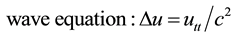 (3)
(3)
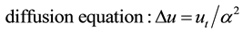 (4)
(4)
The method of separation of variables allows us to isolate the spatial dependence of u from the temporal dependence. Let![]() , substituting this into the wave equation produces
, substituting this into the wave equation produces
![]() (5)
(5)
![]() (6)
(6)
The substitution into diffusion equation leads to the same result. The solution of Equation (6) is a set of eigenvalues ![]() and a set of eigenfunctions
and a set of eigenfunctions ![]() which can be thought as fundamental vibration modes.
which can be thought as fundamental vibration modes.
Finite Element Method
We do not have an equation describing a differentiable variety M, thus we work with a discrete representation of a triangulated surface S described by an OFF file. We need a numerical integration method to solve Equation (6) on S. We have opted to use the Finite Element Method [2] .
First of all, we choose N linearly independent form functions ![]() as a basis of a vector space. These base functions
as a basis of a vector space. These base functions ![]() are chosen to simplify the calculations, so they are constructed as linear functions that “sample” function f at each vertex of the triangulated surface:
are chosen to simplify the calculations, so they are constructed as linear functions that “sample” function f at each vertex of the triangulated surface:
![]() (7)
(7)
The function f then can be written as a linear combination of these base functions
![]() (8)
(8)
The substitution of this approximation in (6) reduces the equation to a generalized eigenvalue problem.
![]() (9)
(9)
where the entry Ui is the contribution of f at vertex i on S. The components of matrix A are given by:
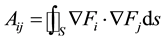 (10)
(10)
and the components of matrix B are:
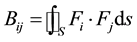 (11)
(11)
Figure 1(a) and Figure 1(b) show the first and second eigenfunctions, respectively, of Equation (9) applied on a triangulated surface of a rat-hippocampus. The lower values are colored in blue and the higher ones in red. We can see the monotonous behavior of the first function whereas the second function grows from the middle of the surface through its extremes.
4. The Construction of the Skeletons
The first step is to transform the OFF format into a graph, in this way we can use standard Graph Theory methods. Let be , the vertices V are indexed as they are in the OFF file, and the edges E can be easily obtained from the list of faces.
We chose the adjacency lists representation for simplicity and efficiency on a triangulated surface with thousands of vertices, usually each one is adjacent only up to five or six vertices; although that number depends on the triangulation and the surfaces. Table 2 shows the adjacency lists of the unitary cube above.
Although the graph is undirected, we allow redundancy of edges in order to simplify the search for local maxima and minima of the eigenfunctions.

 (a) (b)
Figure 1. First (a) and second (b) eigenfunctions on a hippocampus surface.
Table 2. Adjacency lists for the unitary cube.
We do not want to modify the OFF files, so we use an auxiliary file with the values of the first eigenfunctions calculated for each vertex, this is done with the method described in the previous section. On the surfaces studied, we have observed that each eigenfunction gives different information:
・ The first eigenfunction f1 has one maximum and one minimum at opposite points of the surface, these extreme points give us a principal axis, and a main direction (Figure 1(a)). So we decide to use this function to build a polygonal skeleton, which can give us information about curvature and torsion.
・ The second eigenfunction f2 has several local maxima and minima at the prominent protuberances of the surface (Figure 1(b)). So we decide to use this function to build a tree-based skeleton that captures the arborescent structure of the surface.
So we need two variations of the same algorithm, one for each eigenvalue.
4.1. First Eigenfunction Skeleton
Let M and m be the vertices with the absolute maximum and minimum values of the first eigenfunction:  and
and , respectively. We define a set of energy levels
 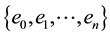 equally spaced:
 (12)
(12)
The vertices fall between these energy levels, however there are some edges with one vertex in one level and the other in the following, so we define a boundary as a subgraph :
:
 (13)
(13)
These boundaries generate a partition of the original graph.
We perform a deep-first search to find one vertex in the boundary Bi, and a second deep-first search to get all the vertices in it. It is possible that for some energy levels these are so close to each other that the algorithm cannot find a definite boundary; in this case we skip to the next level.
Each boundary Bi is a “ring” of vertices, which must be reduced into a centroid ci that can be calculated as a “center of mass”:
 (14)
(14)
where rj represents the coordinates of the vector of vertex j. Obviously, the boundaries for em and eM have just one vertex, so  and
and .
.
Finally we connect these centroids to build the skeleton; this last step is performed by the Prim’s algorithm [8] . This algorithm finds the minimum cost-spanning tree of the set of centroids ci, using their Euclidean distances as the costs function. Although the skeleton for the first eigenfunction is a polygonal, it can be seen as a degenerated tree (a one-degree tree).
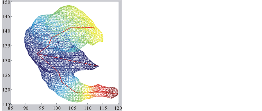
Figure 2(a) and Figure 2(b) show the first eigenfunction skeletons of two surfaces for 32 energy levels.
4.2. The Second Eigenfunction Skeleton
As we exposed for the first eigenfunction, we search for the absolute maximum and minimum points  and
and  and, in this case, we also search for local minima and maxima. A local maximum (or minimum) is a vertex l which is surrounded by vertices of lower (or upper) values of f2.
 (15)
(15)
The search can be easily done in the adjacency lists of E.
We use the coordinates vectors of these vertices as the base of the centroids set:
 (16)
(16)
We define the energy levels ei as in (12) and the boundaries Bi as in (13). However each one of these boundaries could have k connected components , each one has its own centroid
 , as defined in (14). The algorithm for the second eigenfunction process the surface as a tree structure: it performs a deep-first search for a set of boundaries with their respective branch of centroids, and then it performs a second search to find a second branch, an so on. The partition of the surface defined by the first search avoids the algorithm to fall into the same boundaries.
In this case, the Prim’s algorithm shows all its performance in the construction of the skeleton, connecting the set of centroids as a minimum-cost spanning tree. In order to avoid that the skeleton cuts the surface, we add directions to the distances between centroids. We associate the information of the energy level to each centroid:
 (17)
(17)
 (18)
(18)
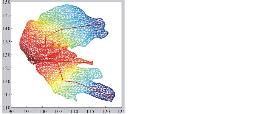
The algorithm connects the centroids in increasing order of . Figure 3(a) and Figure 3(b) show the second eigenfunction skeletons of the same surfaces as Figure 2 and Figure 3.

 (a) (b)
Figure 2. Skeletons of the first eigenfunction on hippocampus (a) and hippocampus (b).
 (a) (b)
Figure 3. Skeletons of the second eigenfunction on hippocampus (a) and hippocampus (b).
5. Conclusions and Further Work
We have developed the algorithms for building the skeletons for the first and second eigefunctions of the Laplace-Beltrami operator calculated on an rat-hippocampus surface depicted by an OFF file.
The skeleton for the first eigenfunction is built as a polygonal structure along the main axis of the surface. The skeleton for the second eigenfunction has a tree-structure with two main branches, each one with a similar structure to the first skeleton, and small branches for some local maxima at prominent protuberances.
This is a first step for the developing of a classification system. The next steps are to generalize these results for different anatomical structures, and define characterization methods for these skeletons based on their geometrical and topological properties, such as critical points of curvature and torsion, bifurcation points, number of branches, etcetera.
References
- Reuter, M., Wolter, F.E. and Peinecke, N. (2006) Laplace-Beltrami Spectra as “Shape-DNA” of Surfaces and Solids. Computer-Aided Design, 38, 342-366. http://dx.doi.org/10.1016/j.cad.2005.10.011
- Reuter, M., Biasotii, S., Patanè, G. and Spagnulo, M. (2009) Discrete Laplace-Beltrami Operators for Shape Analysis and Segmentation. Computer & Graphics, 33, 381-390. http://dx.doi.org/10.1016/j.cag.2009.03.005
- Sadleir, R.J.T. and Whelan, P.F. (2005) Fast Colon Centerline Calculation Using Optimized 3D Topological Thinning. Computerized Medical Imaging and Graphics, 29, 251-318. http://dx.doi.org/10.1016/j.compmedimag.2004.10.002
- Cornea, H.D., Siver, D. and Min, P. (2005) Curve-Skeleton Applications. IEEE Visualization, 23-28 October 2005, 95-102.
- Seo, S., Chung, M.K., Whyms, B.J. and Vorperian, H.K. (2011) Mandible Shape Modeling Using the Second Eigenfunction of the Laplace-Beltrami Operator. Proceedings of SPIE, Medical Imaging, 2011: Image Processing, 7962, 79620Z. http://dx.doi.org/10.1117/12.877537
- Object File Format (2005) Princeton Shape Benchmark. http://shape.cs.princeton.edu/benchmark/documentation/off_format.html
- Thompson, P.M., Hayashi, K.M., et al. (2004) Mapping Hippocampal and Ventricular Change in Alzheimer Disease. Neuroimage, 22, 1754-1766. http://dx.doi.org/10.1016/j.neuroimage.2004.03.040
- Aho, A.V., Hopcfort, J.E. and Ullman, J.D. (1983) Data Structures and Algorithms. Addison-Welsey, Boston.