Applied Mathematics
Vol.4 No.3(2013), Article ID:29091,14 pages DOI:10.4236/am.2013.43080
Importance of Generalized Logistic Distribution in Extreme Value Modeling
1Department of Mathematics, Indian Institute of Science, Bangalore, India
2Department of Statistics, University of Calicut, Calicut, India
Email: nidhin@math.iisc.ernet.in, ccheruvalath@gmail.com
Received September 10, 2012; revised February 1, 2013; accepted February 8, 2013
Keywords: Financial Risk Modeling; Stock Market Analysis; Generalized Logistic Distribution; Generalized Extreme Value Distribution; Tail Equivalence; Maximum Stability; Random Sample Size; Limit Distribution
ABSTRACT
We consider a problem from stock market modeling, precisely, choice of adequate distribution of modeling extremal behavior of stock market data. Generalized extreme value (GEV) distribution and generalized Pareto (GP) distribution are the classical distributions for this problem. However, from 2004, [1] and many other researchers have been empirically showing that generalized logistic (GL) distribution is a better model than GEV and GP distributions in modeling extreme movement of stock market data. In this paper, we show that these results are not accidental. We prove the theoretical importance of GL distribution in extreme value modeling. For proving this, we introduce a general multivariate limit theorem and deduce some important multivariate theorems in probability as special cases. By using the theorem, we derive a limit theorem in extreme value theory, where GL distribution plays central role instead of GEV distribution. The proof of this result is parallel to the proof of classical extremal types theorem, in the sense that, it possess important characteristic in classical extreme value theory, for e.g. distributional property, stability, convergence and multivariate extension etc.
1. Introduction
An important problem from the field of stock market modeling is the determination of adequate model for extreme stock movement. In financial literature, the choice of using an appropriate probability model for financial returns are clearly exemplified rather than selecting a conventional model (see for ex. [2]). The fitted tale distribution is crucially important in financial studies. For Value at Risk (VaR) estimation, one requires appropriate probability distribution of extremes as input. A vast number of literature show the importance of best fitted distribution in VaR analysis (see [3]). Another important area of application of probability models of extremes is in hedging procedure. Hedging procedure is clearly based on the probability of fitted distribution (see [4]). Also measuring the risk attached to a share or portfolio will critically depends on the tale distribution. [5] largely illustrates the importance of appropriate probability models for extremes of financial returns data.
Initially, normal and lognormal distributions were used to model data which arise from financial sector. In the last five decades, different authors have been showing that the distribution of extreme daily returns is far from normal (see [5-11]. They used a number of distributions different from normal and lognormal to model large values of finance data. For example t-distribution, alpha stable distribution, etc. In 1990’s the interest in modeling large values of finance data have been diverted to extreme value theory where modeling maximum of the data, generalized extreme value distribution for maxima (GEV (max)) or generalized Pareto (GP) distribution are used and for minimum of the data, generalized extreme value distribution for minima (GEV(min)) is used. These distributions enjoy strong theoretical support for analyzing extreme movement of a data compared to other models. Below we give an outline of these theoretical properties of the distributions.
The theoretical representation for GEV(max) and GEV(min) have been established by Jenkinson and Von Mises (see von Mises (1954) and Jenkinson (1955)). We define GEV(max) below.
Definition 1.1 A random variable X is said to follow the generalized extreme value distribution for maximum (GEV(max)) if its distribution function is given by,
and the supports are
The related location-scale family can be introduced by replacing the argument  above by
  for
for 
and . The parameter
  is known as the shape parameter of the distribution and different values of
  leads to different well known distributions. That is, for
 , it is the Gumbel (Type I) distribution which is interpreted as
 , For
, For , it is the reverseWeibull (Type III) distribution, for
 , it is Frechet (Type II) distribution. Also GEV(min) can be defined as follows.
Definition 1.2 A random variable X is said to follow the generalized extreme value distribution for minimum (GEV(min)), if its distribution function is given by,

and the supports are

The parameter  is the shape parameter and
 . One can introduce the related location-scale family by replacing the argument x above by
  for
for 
and . For
. For  (which is interpreted as
 ), the distribution is called reverse-Gumbel, for
 , it is called reverse-Frechet distribution and for
 , the distribution is the Weibull distribution.
The above two distributions possess the characterizing properties called max-stability and min-stability respectively. In the following we define max-stability for nonrandom sample size.
Definition 1.3 A non-degenerate random variable  is said to be max-stable if, for each
  there are constants
  and
and  such that
where  are same copies of
 .
.
Similarly, one can define min-stability. By the extremal types theorem, asymptotic distribution of maxima of independent and identically distributed random variables (i.i.d.r.v.’s) under proper normalization can be approximated by the GEV(max) distribution. Below we give an outline of the theorem.
Theorem 1.1 (see [12]): Let  be a sequence of i.i.d.r.v.’s and
 . If there exist sequences of norming constants
  , and a non-degenerate d.f.
  such that,
 (1.1)
(1.1)
then , in Equation (1.1), is the GEV(max) distribution defined in Definition 1.4.
Since , the asymptotic distribution of minima of i.i.d.r.v.’s can be derived as
 , where
  is the GEV(max). Hence the asymptotic distribution for minima is the GEV(min) distribution defined in Definition 1.2. These theories have been extended to multivariate case, where multivariate generalized extreme value distributions play central role (see [13,14]).
Another alternative model for maxima is the generalized Pareto distribution, has been suggested by two independent works [15] and [16]. Below we define GP distribution.
Definition 1.4 A random variable X is said to follow the generalized Pareto (GP) distribution if its distribution function is given by,
and the supports are
The parameter  is the shape parameter and
 . One can introduce the related location-scale family by replacing the argument
  above by
  for
for 
and . With respect to
 ,
,  and
and  we get the exponential distribution, beta distribution and Pareto distribution.
GP distribution possess characterizing property called Peak over Threshold (POT) stability w.r.t non-random sample size. In the following we define POT stability for non-random sample size.
Definition 1.5 A non-degenerate random variable  is said to be POT-stable if, for each
  there are constants
  and
and  such that
By Peak over threshold theorem, under proper normalization, the asymptotic distribution of the observations above exceedances of a level u has a generalized pareto distribution iff asymptotic distribution of maximum of the observations, under proper normalization, is the GEV(max) distribution. We give an outline of the theorem below.
Theorem 1.2 (see [15,16]) let  be a sequence of i.i.d.r.v.’s with common continuous distribution function
 . Suppose there exists a pair of sequences
  and
and  with
with  for all
  and a non-degenerate distribution function
  such that
 (1.2)
(1.2)
for all  at which
  is continuous. Let

Then, under proper normalization,  can be approximated by generalized Pareto (GP) distribution, when
  (where
 ).
).
This theory also extended to multivariate case, where multivariate generalized Pareto distribution plays central role (see [17]).
Extremal types theorem (see [18]) and Peak over threshold theorem ([15,16]) facilitate a theoretical background to use generalized extreme value (GEV) distributions and GP distribution in modeling extreme movement of stock market indices. A number of researchers verified empirically that these models give sufficient fit to model extreme volatility in stock market, see for ex. [19,20]. Also many researches utilizes these models for measuring extremal behavior of stock markets, see for ex. [4,21,22].
However, from 2004, [1] and many other researchers have been empirically showing that generalized logistic (GL) distribution is a better model than GEV and GP in modeling extremal behavior of different stock market data, this includes US, UK, Germany, Japan, India, Athens, African stock markets etc. See for eg. [1,23,24] etc. Also [25] empirically showed that GL is better than GEV to model extreme movements in the stock, commodities and bond markets.
In this paper we show some theoretical motivation of this claim, that is, we present a theoretical framework of the role of GL distribution in extreme value modeling. In Section 2, we define logistic distribution and some of the known results of the logistic distribution which are important in extreme value theory. We also define generalized logistic distribution in this section. Section 3 introduces some of the notable properties of GL distribution, namely, tale equivalence with GEV and GP distributions and stability property w.r.t geometric distribution. We prove a general multivariate limit theorem in Section 4, and show multivariate central limit theorem, multivariate extremal types theorem and multivariate random sum convergence theorem are special cases of this theorem. In Section 5, we use the above general limit theorem to prove the convergence of random maxima and random minima to GL distribution. For an additional support to our claim, we present a data analysis in Section 6. We introduce a multivariate generalized logistic distribution in Section 7, and also we prove a characteristic property of this multivariate distribution by using the general multivariate theorem in Section 4.
To prove the results we require some basic concepts which we discuss below.
Definition 1.6 The right end point and left end point of a d.f. , denoted by
  and
and  respectively, are

Definition 1.7 Two distributions F and G are equivalent in their right tail if they have the same right end point, i.e. , and
, and

Definition 1.8 Two distributions F and G are equivalent in their left tail if they have the same left end point, i.e. , and
, and
For more details see [26]. Next, we introduce the maxstability w.r.t. a discrete distribution.
Definition 1.9 (see [27]) Let  be a non-degenerate distribution function of a random variable
  and
and  be a discrete random variable defined on set of positive integers with probability mass function
 . That is,
Then  is said to be max-stable w.r.t.
  (or r. v.
  is said to be maximum stable w.r.t. a r. v.
 ) if there exist
  and
and  such that,
where  are same copies of
 .
.
Similarly, one can define min-stability w.r.t. a discrete distribution.
2. Review of Logistic and Generalized Logistic Distribution
Logistic distribution is an important distribution used in statistical modeling. It is used for modeling in a number of research papers (see [28]). In literature, Logistic distribution plays some important role in modeling of extremes of data. In this section, first, we define Logistic distribution and then discuss its importance in extreme value theory.
Definition 2.1 A random variable X is said to follow standard logistic distribution if its d.f is given by
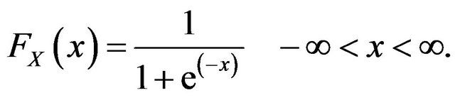 (2.1)
(2.1)
The following are some important results which connects logistic distribution and extreme value theory.
Result 2.1 ([27]): Let  be a sequence of i.i.d.r.v.s with symmetric distribution function
 . Let
. Let  be an integer valued random variable independent of
  and
and
 (2.2)
(2.2)
Let  and there exist constants
  and
and  such that
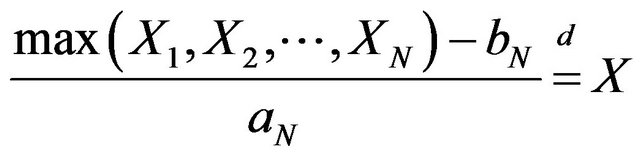
iff  is the logistic distribution function.
The logistic distribution appears as a limiting distributions as described in the following result.
Result 2.2 (see [28]): Let  be a sequence of independent and identically distributed random variables with distribution function
 . Let
. Let  be a integer valued random variable which are not necessarily independent of
 . Assume
  is in the domain of attraction of Gumbel distribution and
where  is a proper distribution function. Then the limit distribution of
  is logistic iff
 .
.
The next result brings the connection between logistic distribution and the extreme value theory through midrange.
Result 2.3 (see [28]): Let  be a sequence of independent and identically distributed random variables with
  follows
 . Let
. Let
 and
and
 . Assume
  is symmetric distribution which belongs to the domain of attraction of Gumbel distribution then under proper normalization the midrange
converges to the random variable  which follows standard logistic distribution given in Definition 2.1.
In statistics literature, there are several ways of generalizing the logistic distribution (for more details see [29]). Among the various generalization of logistic distribution, the one given by Hosking (see [30]) is called the 5th generalized logistic distribution ([29]). This form of generalized logistic distribution is used for many real life applications, see for example [1,23,24,30,31]. Motivated by this we introduce the 5th generalized logistic distribution and call this generalization of logistic distribution as generalized logistic distribution.
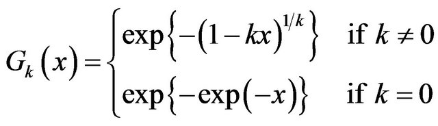
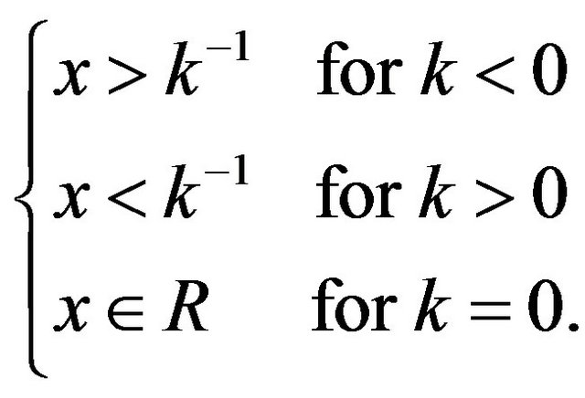
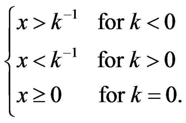
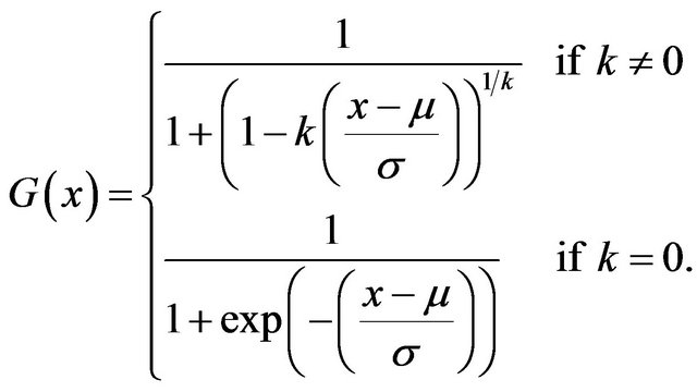
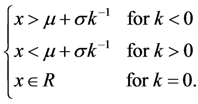
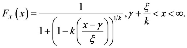
Definition 2.2 A random variable X is said to follow the generalized logistic (GL) distribution if its distribution function is given by,
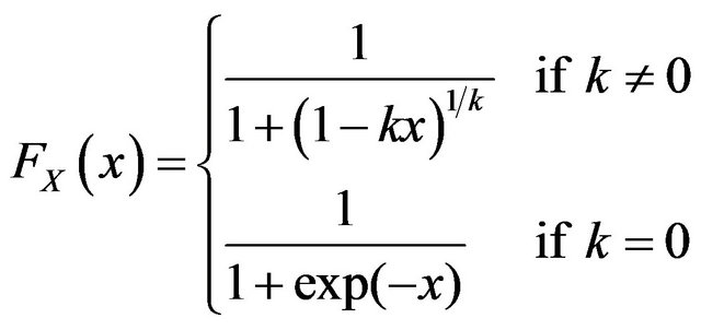
and the supports are

The parameter  is known as the shape parameter of the distribution and
 . One can introduce the related location-scale family by replacing the argument
above by  for
for  and
and . For k = 0,
can be identified as the logistic distribution. For , and some scale transform, we get loglogistic distribution as given in [27]. Similarly for
 , through some scale transform we get backward loglogistic distribution. The statistical properties and estimation issues of the GL distribution are discussed in [29].
3. Some Notable Properties of GL Distribution
In this section we prove some characters of GL distribution which are important to extreme value theory. We study the tail behavior of GL distribution compared to other distributions. Also, as we see in GEV and GP distributions, we prove GL distribution is also characterized by a stable property.
3.1. Tail Equivalence of GL, GEV and GP
In this subsection, we compare tail distribution of GL with GEV(max), GP and GEV(min). Figures 1 and 2 gives the probability density functions and distribution functions of GL, GEV(max), GP and GEV(min) for k = 0 respectively. Figures 1 and 2 indicate that the right tails of the GEV(max), GP and GL distributions are similar and GEV(min) and GL are similar in left tails. This clearly indicates that these three distributions are asymptotically
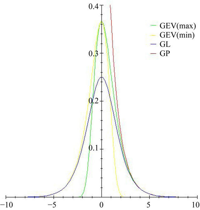
Figure 1. Probability density functions of GEV(max), GEV(min), GP and GL distributions.

Figure 2. Distribution functions of GEV(max), GEV(min), GP and GL distributions.
equivalent in their tails, which we prove in the following theorems.
Theorem 3.1 The distributions GEV(max), GP and GL are equivalent at their right tails. The distributions GEV(min) and GL are equivalent at their left tails.
3.2. Max-Stability and Min-Stability w.r.t Geometric Distribution
From Result 2.1, the logistic distribution is characterized by max-stability property. Here we prove the property still remains with this generalization. Below theorem show that the GL distribution also characterized by maxstability and min-stability w.r.t geometric distribution.
Theorem 3.2 The generalized logistic distribution given in Definition 2.2 characterizes max-stability w.r.t geometric distribution. That is, let  be a sequence of i.i.d random variable follows GL distribution if and only if there exist real numbers
  and
and  such that,

where N is a discrete random variable follows geometric distribution. Similarly, the result is true for minimum.
Hence GL satisfies the stability property. In the next Section we prove a theorem which gives a direct relation between stability property and limit distribution of a general class of functions. We use this theorem to prove a limit theorem in extreme value theory where GL plays the central role.
4. A General Multivariate Limit Theorem
Here we prove a limit theorm of general functions of independent identically distributed continuous multivariate random variables (i.i.d.c.m.r.v) which posses property Q
(see Definition 4.1). Let  be a Borelmeasurable function of
 , which is continues. We use the multivariate norming function as
 .
.
Below we define a property  of a Borel measurable function.
Definition 4.1 Let  be a Borelmeasurable function then g satisfies property
  if,
if,

where  and
and  are integer valued random variables or integers such that
 .
.
The functions 
are some of the important examples of functions which satisfy Property Q. By  we mean the coordinate wise maximum. These functions with random sample size also satisfy Property Q, for more details see [32].
Theorem 4.1 Let 
be a sequence of i.i.d.c.m.r.v and  be a Boral-measurable function such that
  satisfies property
 , and
, and  is independent of each
 . Let
. Let  be a non-degenerate r.v. Then there exists sequences
  and
and  such that
iff Y satisfies the following equation
for some sequences  and
and , where
  are same copies of
 .
.
Many important limit theorem in probability can be deduced as a special cases of Theorem 4.1, which includes multivariate central limit theorem, multivariate extremal types theorem and Random Sum Convergence theorem, which we show in the following subsections.
4.1. Multivariate Version of Generalized Central Limit Theorem as a Special Case
Let η = n and , then g satisfies property Q as described in Definition (4.1). Let X be the class of random variables which follows multivariate stable distributions. Then for all
  there exist a sequence
  and
and  such that, for each n,

where  are same copies of
 , see [11]. Let
  be an i.i.d sequence of r.v’s and
  be a non-degenerate r.v. Then there exist
  and
and  such that
iff .
.
4.2. Multivariate Extremal Types Theorem as a Special Case
Let  and
and
 , then g satisfies property
 . Let
. Let  be the class of random variables follows multivariate extreme value distributions with characterizing property,
where  are same copies of
 . Let
. Let  be a sequence of i.i.d.c.m.r.v’s and
  be a non-degenerate r.v. Then there exist
  and
and  such that
iff .
.
4.3. Random Sum Convergence as a Special Case
Let , a r.v and
 , then
 satisfies property
 . Let
. Let  be the class of random variables which follows multivariate strictly geometric stable distribution. Then for all
  there exist constants
  and
and  such that, for each n,
where  are same copies of
 , see [33,34]. Let
  be an i.i.d sequence of r.v’s and
  be a non-degenerate r.v. Then there exist
  and
and  such that
iff .
.
5. GL as a Limit Distribution of Random Maxima and Minima
The limit theory of random maxima and random minima has been studied by many authors (see for ex. [35]). In this section we derive generalized logistic distribution as the limit of random maxima and random minima when sample size follows geometric distribution using Theorem 3.2 and 4.1.
Theorem 5.1 Let  be a sequence of i.i.d.c.r.v. Let
 ,
,
 , and N is an integer valued random variable which follows geometric distribution, independent of
 . Also let
  and
and  be random variables with non-degenerate distribution functions
  and H respectively,
  ,
,  ,
,  and
and  such that,

and
Then
with supports are
also  has the same distributional form of
  with different parameters.
Proof. The proof consist of two parts. First, from Theorem 3.2, it is verified that GL posses characterizing property of max-stability and min-stability w.r.t geometric distribution. By using Theorem 4.1, where the random maxima and random minimum, when sample size follows geometric distribution, converge to the GL distribution, if it exists.
Theorem 5 identifies the limit distribution of geometric random maxima and geometric random minima, if it exists, as the GL distribution given in Section 2.2. That is, GL distribution can be used as an asymptotic model for maximum and minimum of a random number  of random variables, when N follows geometric distribution. Notably, unlike of GEV(max), GEV(min), and GP, GL distribution provides the theory for both maxima and minima. This is an alternative model for maxima and minima. The theory is parallel to generalized extreme value model and generalized Pareto model in the sense that the three models includes three important distributions which is decided by the shape parameter. Also tail of these models are asymptotically equivalent and three models have a characterizing stability property in different sense. Moreover, the three models can be considered as the limit distribution of extremes in different situations. These results justify the theoretical importance of the empirical findings, that GL can be a suitable model over GEV model for extremes of share market data, see for example [1,25,26]. Many papers also show that GL distribution provides an adequate distribution in hydrological application, for eg. [30,31] etc.
Remark 5.1 It is also be noted that this theorem is somewhat similar to geometric stable theorem in the theory of partial sum of random variables where geometric stable (GS) distribution plays a central role. GS distribution is widely using in stock market modelingand GS can be viewed as the weak limit distribution of sum of random number of random variables, whose random number follows geometric distribution.
6. Goodness of Fit Test for the BSE Data
In this section, we empirically study the performance of GL and GEV in modeling the behavior of minimum returns of Bombay stock exchange data. We use AndersonDarling test for comparing goodness of fit of GEV and GL distributions in the extremal behavior of the data. Since the test is based on empirical distribution function (EDF) and among all the well known tests based on EDF, Anderson-Darling test has the highest power in testing normality against a number of alternatives when the parameters are unknown [36].
Table 1 shows a comparison between performance of GEV(min) and GL on minima returns. For fifteen intervals, GL provides an adequate fit in eleven intervals than GEV(min), which indicates that GL distribution provides a better fit than GEV(min). However, GEV(min) provides an adequate fit in 11 out of 15 intervals and in which most of the intervals p-values are large, which shows that GEV(min) also provides a model for minimum returns.
Table 2 shows that GL provides a better fit in six interval compared to GEV(min). While GEV(min) provides an adequate fit in nine out of ten intervals showing that GEV(min) is also a model for monthly minima.
Comparing GL and GEV(min) in quarterly minimum data, Table 3 indicates the same result, that is, GL provides a better fit than GEV(min). Further GEV(min) and
Table 1. Performance of GEVmin and GL distribution for weekly minimum data.

Table 2. Performance of GEVmin and GL distribution for monthly minimum data.
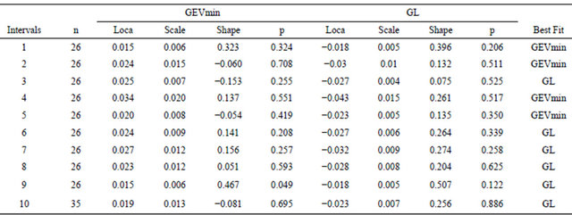
Table 3. Performance of GEV(min) and GL distribution for quarterly minimum data. *Indicates neither distribution fit the data.
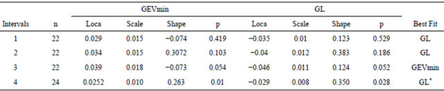
GL gives a good model in three out of four intervals, which shows both distribution can be used to model quarterly data and comparing these distributions GL is a better model.
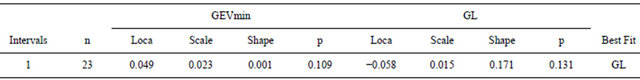
On analysis of half yearly data, Table 4 clearly shows GL provides a good fit comparing to GEV(min). Finally, Table 5 illustrates GL provides a better for yearly minimum data compared to GEV(min). Both distribution fit for the data at 0.05 level.
The above analysis reveals that for analyzing the minimum returns in stock market data, GL provides a better fit than GEV distributions, which shows minimum behaves like a geometric minimum than the usual minimum in stock market data (for more details see [37]).
7. Multivariate Generalized Logistic Distribution and a Characterization Property
In Section 5, we identified that GL distribution is also a suitable model for extremes, moreover it plays better model than GEV in some situations. We also proved that the above theorem is parallel to the existing extremal types theorem and peak over threshold theorem. Naturally, one can think a multivariate version of GL distribution as parallel to the theory of multivariate extreme value distribution.
Definition 7.1 Let 
be a sequence of i.i.d.c.m.r.v and let
 , where N is random variable follows geometric distribution. Let
  and
and  are p-dimensional real sequences such that
Suppose the following convergence occur,
Then we called  as multivariate generalized logistic (MGL) distribution and
 , where
is the domain of attraction of .
.
Notice that, the univariate margins of G must be a generalized logistic distribution, this includes all three types of the marginal distribution: k = 0, k > 0 and k < 0 correspond respectively to the logistic, loglogistic and backward loglogistic distributions. Below we prove a characterizing property of MGL distribution.
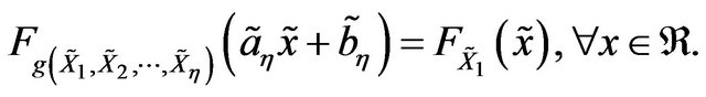
Theorem 7.1 The MGL distribution is characterized by max-stability w.r.t geometric distribution. That is, let  be a random variable follows geometric distribution.
Table 4. Performance of GEV(min) and GL distribution for half yearly minimum data.
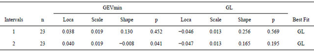
Table 5. Performance of GEV(min) and GL distribution for yearly minimum data.
let  be a sequence of i.i.d.c.m.r.v which follows MGL distribution iff there exist
  and
and  are p-dimensional real sequences such that

and,

Proof. The result is directly from Theorem 4.1.
7.1. Proof of Theorem 3.1
Since the proof contains only simple calculation, we only give proof for tail equivalence of GEV(max)and GP. We use notations  and F for distribution functions of GEV(max)and GL respectively.
As per the assumed notation for the distributions of GEV(max) and GL, to prove the asymptotic equivalence of their right tails, by Definition 1.7, it is enough to prove that  and
and

We prove this in the following three cases.
Case 1 . Here
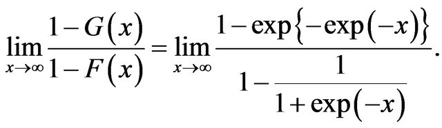
This is  form. So applying L-Hospital’s rule we get,
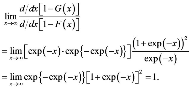
Case 2 . Here also
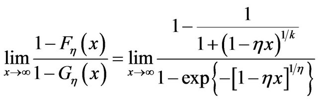
which is again  form. So applying L-Hospital’s rule,

Case 3 . In this case

7.2. Proof of Theorem 3.2
To prove the max-stability of GL, we use the following lemma from [27].
Lemma B.1 Let  be a non-degenerate distribution function of a r.v.
  which is maximum stable w.r.t
 . If
. If ,
,  , and for any real constant
 , and d.f’s
  and
and  defined by
 and
and
 for all real
 , then
  and
and  are non-degenerate and maximum stable w.r.t
  with
with  and
and  respectively.
For detailed discussion see [27]. Below we prove Theorem 3.2.
Proof. Let  be the distribution function of generalized logistic distribution with
 , and location and scale parameters
  and
and  respectively. That is,
Now take the transformation , we get,
which is the distribution function of Logistic distribution (see [27]). That is,  is logistic distribution function and by Lemma (B.1), the distribution function
  is max-stable w.r.t geometric distribution. Similarly, for
 , the same proof works. That is, GL distribution satisfies max-stability w.r.t geometric distribution. To prove that GL is the only distribution with property of max-stability, let
  be a random variable which follows GL distribution with shape parameter
 . Now take the transformation
 (5)
(5)
then for ,
,  follows loglogistic distribution with distribution function
where  and
and . For
. For , Y follows backward loglogistic distribution. By [27], we know that the class containing logistic, loglogistic and backward loglogistic has the characterizing property max-stability w.r.t to geometric distribution. The relation (B.1) is one to one implies the max-stability property w.r.t to geometric distribution characterize generalized logistic distribution. Similarly we can prove that min-stability characterizes GL distribution w.r.t geometric distribution.
Remark B.1 In the above proof, we give short steps mainly using Voorn’s idea (see [27]). One can directly prove the theorem.
7.3. Proof of Theorem 4.1
Let  be a sequence of independent and identically distributed continues multivariate random variables (i.i.d.c.m.r.v) defined on some probability space
 . We use symbols
 ,
,  and
and  to denote both non random integer and integer valued random variable, particularly, we write
  when we consider non random integer and N, depends on some parameter
 , for integer valued random variable. When
 , non-random, then
  may be interpreted as
 . To prove the theorem we need the following
  function in multivariate case.
Definition C.1 Let  be a sequence of i.i.d.c.m.r.v with
  represents distribution function of
  and
and  be a given Borel function. Define,
and for every value of , where
  is a positive integer, we get
Also the cardinality of  and
and  are same. Let
  be a sequence of class of functions such that,

Then for every value of ,
,  a
a  such that,
 (C.1)
(C.1)
Below we give a simple example of the above  function.
Example C.1 Let  be a sequence of i.i.d.c.m.r.v and
 is given. Then the function
  is,
is,

Remark C.1 Let  and
and  be given sequences and let
  be the following form,

which implies,
also  and
and  can define accordingly.
In the following we prove Theorem 4.1.
Proof. Let  be a non-degenerate distribution function. Let
  be a sequence of i.i.d.c.m.r.v such that
  (for notational convenience we use
  instead of
 ) and define
be the class of sequences of distribution functions which convergence to . We use the notation
for a member  in
in . Now, we define a Function space
 , w.r.t
 , as
, as

with a matric  as
as
 (C.2)
(C.2)
where  is from
and  are particular values of
 . It is easy to verify
  follows metric conditions on
 . We denote
 for
for .
.
Next we define a relation  on
on . That is, let
 ,
,  and
and  are three sequence of random variables each forms i.i.d and
 ,
,  and
and . Now let
 . We say that
  and
and  are
are 
related (denoted by ) if
) if
 (C.3)
(C.3)
Then below we show that the relation  is an equivalence relation on
 . Let
. Let . Since
the relation is reflexive. Also let 
and . That is,
implies
or  so that the relation is symmetric. Now let
  and
and , such that
  and
and  That is,

and
Then,

that is  is transitive.
So we have a partition on  by the equivalence relation
 .
.
Now we show that  always exists and is a graph of a distribution function. Clearly for any
  then
then
 and
and
 . Also
  is one to one and onto function and each of its variable the function is monotone implies
  monotonically non decreasing for each of its variable and and right continuous for each of its coordinates.
Then we prove the following equation,
 (C.4)
(C.4)
Let  be i.i.d.c.m.r.v’s and
 be a Borel measurable function. Now for
 , define
then  is also a sequence of i.i.d.c.m.r.v’s. Let
 and
and . Then

which is same as,
But we know that
Hence,
But  So by property
 (C.5)
(C.5)
Now we can show existence of a special property in the function space. That is, there exist a special member, we call this member as stable member, in each equivalent class.
Given that in every equivalent class, there exist at least one  such that

which implies

for every . By using Equation (C.5) we get
That is,
Putting  we get
then by using multivariate version of Khintchine’s theorem, there exist sequence  and
and  such that

Here we need the assumption of weak convergence. Which implies
 (C.6)
(C.6)
So that  satisfies stability property.
Now, we have a partition on  and we know that every equivalent class contains a stable member. let
  be one of the equivalent class introduced by the relation
  and
and  is a stable member in
 . That is,
Then for all ,
,
 (C.7)
(C.7)
Since, 
 implies,
But

The above two equation implies,

Therefore,
Hence, in the function space, every equivalent class contains at least a stable member and all other members of that class will converge to that stable member. It is easy to prove that the limiting member is unique in every class, if it exist. This complete the proof.
Remark C.2 In Equation (C.6), we introduce a property called multivariate stability property for some of the members in . This is a multivariate extension of stability property in [32]. Below we give an exact definitions and some examples of this property.
Definition C.2 Let  be a given one to one functions. We say that
  satisfies stability property if it is a constant sequence in
 . In other words,
  satisfies stability property if for each
 ,
,
That is for each ,
,
A member  is called a stable member if it is a constant sequence in
 . Using Equation (C.1) the stability property can be rewritten for sequence
  in terms of the function g as follows.
Definition C.3 Let  be a sequence of i.i.d.c.m.r.v and
  be a Borel function of
 . Then we say that
  satisfies stability property for the given function
  if, for every
 ,
,
Example C.2 Let  be a sequence of i.i.d.c.m.r.v. and
  follows strictly multivariate geometric stable distribution and
  be a random variable, independent of
 , and
, and  follows geometric distribution. Let
 . Then there exist a sequence
 , depends on N, such that
 is a stable member since,
see [38].
Remark C.3 By Equation (C.7), each equivalent class forms the domain of attraction of a stable member.
Below we define domain of attraction.
Definition C.4 Let  be a given one to one functions. Let
 . For any distribution function
  such that
 , we say that
  is the domain of attraction of
  if for every
 ,
,
That is,

Therefor for each stable member, there exist an equivalent class of  which is the domain of attraction of the stable member. Below remark gives a distance measure between domain of attractions.
Remark C.4 Let  be the class of all domain of attractions for a given sequences of functions
 . Then
  is a complete metric space with metric
 , which is defined as, if
  and
and  are two elements of
 , then
where  and
and
 . For the proof see Theorem 27 in [39] and a complete proof see Page (202,203) in [40].
8. Acknowledgements
This work is supported in part by Dr. D.S. Kothari Fellowship of UGC and in part by UGC-DSA SAP-Phase IV.
REFERENCES
- G. D. Gettinby, C. D. Sinclair, D. M. Power and R. A. Brown, “An Analysis of the Distribution of Extremes Share Returns in the UK from 1975 to 2000,” Journal of Business Finance and Accounting, Vol. 31, No. 5-6, 2004, pp. 607-645. doi:10.1111/j.0306-686X.2004.00551.x
- P. Kearns and A. Pagan, “Estimating the Density Tail Index for Financial Time Series,” Review of Economic Statistics, Vol. 79, No. 2, 1997, pp. 171-175. doi:10.1162/003465397556755
- J. Danielson, P. Hartmann and C. de Vries, “The Cost of Conservatism,” Risk, Vol. 11, No. 1, 1998, pp. 103-107.
- J. Cotter, “Margin Exceedences for European Stock Index futures Using Extreme Value Theory,” Journal of Banking & Finance, Vol. 25, No. 8, 2001, pp. 1475-1502. doi:10.1016/S0378-4266(00)00137-0
- E. Fama, “The Behaviour of Stock Market Price,” Journal of Business, Vol. 38, No. 1, 1965, pp. 34-105. doi:10.1086/294743
- J. B. Gray and D. W. French, “Emperical Comparisons of Distributional Models for Stock Index Returns,” Journal of Business, Finance and Accounting, Vol. 17, No. 3, 1990, pp. 451-459. doi:10.1111/j.1468-5957.1990.tb01197.x
- R. D. F. Harris and C. C. Kucukozmen, “The Emperical Distribution of UK and US Stock Returns,” Journal of Business Finance and Accounting, Vol. 28, No. 5-6, 2001, pp. 715-740. doi:10.1111/1468-5957.00391
- B. Mandelbrot, “The Variation of Certain Speculative Prices,” Journal of Business, Vol. 36, No. 4, 1963, pp. 394-419. doi:10.1086/294632
- J. McDonald and Y. Xu, “A generalization of Beta Distribution with Applications,” Journal of Econometrics, Vol. 66, No. 1-2, 1995, pp. 133-152. doi:10.1016/0304-4076(94)01612-4
- A. Peiro, “The Distribution of Stock Returns: Internatinal Evidence,” Applied Financial Economics, Vol. 4, No. 6, 1994, pp. 431-439. doi:10.1080/758518675
- P. Theodossiou, “Financial Data and the Skewed Generalised-T Distribution,” Management Science, Vol. 44, No. 12, 1998, pp. 1650-1661. doi:10.1287/mnsc.44.12.1650
- P. Embrechts, C. Kluppelberg and T. Mikosch, “Modeling Extremal Events for Insurance and Finance,” Springer-Verlang, Berling, Heidelberg, 1997. doi:10.1007/978-3-642-33483-2
- S. Kotz and S. Nadarajah, “Extreme Value Distributions: Theory and Applications,” Imperial Collage Press, London, 1999.
- S. I. Resnick, “Extreme Values, Regular Variation, and Point Processes,” Springer-Verlag, New York, 1987.
- A. A. Balkama and L. de Haan, “Residual Life Time at Great Age,” The Annals of Probability, Vol. 2, No. 5, 1974, pp. 792-804. doi:10.1214/aop/1176996548
- J. Pickands, “Statistical Inference Using Extreme Order Statistics,” The Annals of Statistics, Vol. 3, No. 1, 1975, pp. 119-131. doi:10.1214/aos/1176343003
- H. Rootzen and N. Taijvidi, “Multivarate Generalized Pareto Distribution,” Bernoulli, Vol. 12, No. 5, 2006, pp. 917-930. doi:10.3150/bj/1161614952
- M. R. Leadbetter, G. Lindgren and H. Rootzen, “Extremes and Related Properties of Random Sequences and Processes,” Springer-Verlag, New York, 1983.
- F. M. Longin, “The Asymptotic Distribution of Extreme Stock Market Returns,” Journal of Business, Vol. 69, No. 3, 1996, pp. 383-408. doi:10.1086/209695
- F. M. Longin, “From Value at Risk to Stress Testing: The Extreme Value Approach,” Journal of Banking and Finance, Vol. 24, No. 7, 2000, pp. 1097-1130. doi:10.1016/S0378-4266(99)00077-1
- F. M. Longin, “Stock Market Crashes: Some Quantitative Results Based on Extreme Value Theory, Derivatives Use,” Trading Regulation, Vol. 7, No. 3, 2001, pp. 197- 205.
- A. I. Maghyereh and H. A. Al-Zoubi, “The Tail Behavior of Extreme Stock Returns in the Gulf Emerging Markets: An Implication for Financial Risk Management,” Studies in Economics and Finance, Vol. 25, No. 1, 2008, pp. 21- 37. doi:10.1108/10867370810857540
- K. Tolikas and R. A. Brown, “The Distribution of Extreme Daily Share Returns in the Athens Stock Exchange,” The European Journal of Finance, Vol. 12, No. 1, 2006, pp. 1-12. doi:10.1080/1351847042000304107
- K. Tolikas, and G. D. Gettinby, “Modelling the Distribution of the Extreme Share Returns in Singapore,” Journal of Empirical Finance, Vol. 16, No. 2, 2009, pp. 254-263. doi:10.1016/j.jempfin.2008.06.006
- K. Tolikas, “Value-at-Risk and Extreme Value Distributions for Financial Returns,” The Journal of Risk, Vol. 10, No. 3, 2008, pp. 31-77.
- S. I. Resnick, “Tail Equivalence and Its Applications,” Journal of Applied Probability, Vol. 8, 1971, pp. 135- 156. doi:10.2307/3211844
- W. J. Voorn, “Characterization of the Logistic and Loglogistic Distributions by Extreme Value Related Stability with Random Sample Size,” Journal of Applied Probability, Vol. 24, 1987, pp. 838-851. doi:10.2307/3214209
- N. Balakrishnan, “Handbook of the Logistic Distribution,” Marcel Dekker, New York, 1992.
- N. L. Johnson, S. Kotz and N. Balakrishnan, “Continuous Univariate Distributions,” John Wiley, New York, 1995.
- J. R. M. Hosking and J. R. Wallis, “Regional Frequency Analysis: An Approach Based on L-Moments,” Cambridge University Press, Cambridge, 1997.
- S. Hongjoon, N. Woosung, J. Younghun and H. JunHaeng, “Asymptotic Variance of Regional Curve for Generalized Logistic Distribution,” World Environmental and Water Resources Congress, Great Rivers, 2009.
- K. Nidhin and C. Chandran, “Limit Theorems of General Functions of Independent and Identically Distributed Random Variables,” Statistics and Probability Letters, Vol. 79, No. 23, 2009, pp. 2397-2404. doi:10.1016/j.spl.2009.08.013
- L. B. Klebanov, S. Mitinik, S. T. Rachev and V. E. Volkovic, “A New Representation for the Characteristic Function of Strictly Geo-stable Vectors,” Journal of Applied Probability, Vol. 37, No. 4, 1999, pp. 1137-1142.
- T. T. Nguyen and A. R. Sampson, “A Note on Characterizations of Multivariate Stable Distributions,” Annals of the Institute of Statistical Mathematics, Vol. 43, No. 4, 1991, pp. 793-801. doi:10.1007/BF00121655
- J. Galambos, “The Asymptotic Theory of Extreme Order Statistics,” Wiley, New York, 1978.
- M. A. Stephens, “EDF Statistics for Goodness of Fit and Some Comparisons,” Journal of American Statistical Association, Vol. 69, No. 347, 1974, pp. 730-737. doi:10.1080/01621459.1974.10480196
- K. Nidhin and C. Chandran, “An Analysis of the Extremal Behavior of Bombay Stock Exchange Data,” International Journal of Statistics and Analysis, Vol. 1, No. 3, 2011, pp. 239-256.
- T. J. Kozubowski and S. T. Rachev, “Multivariate Geometric Stable Laws,” Journal of Computational Analysis and Applications, Vol. 1, No. 4, 1999, pp. 349-385. doi:10.1023/A:1022692806500
- J. L. Kelley, “General Topology,” Springer, New York, 1955.
- S. Lipschutz, “General Topology,” Schaum’s Outline Series, New York, 1965. doi:10.1007/978-1-4612-5449-2