Journal of Environmental Protection
Vol. 4 No. 8A1 (2013) , Article ID: 36281 , 7 pages DOI:10.4236/jep.2013.48A1018
Association between Air Cane Field Burning Pollution and Respiratory Diseases: A Bayesian Approach
![]()
Department of Social Medicine, Ribeirão Preto Medical School, University of São Paulo, Ribeirão Preto, Brazil.
Email: achcar@fmrp.usp.br
Copyright © 2013 Jorge Alberto Achcar et al. This is an open access article distributed under the Creative Commons Attribution License, which permits unrestricted use, distribution, and reproduction in any medium, provided the original work is properly cited.
Received June 11th, 2013; revised July 15th, 2013; accepted August 12th, 2013
Keywords: Hospitalization Counting; Bayesian Models; Times between Hospitalization Extrapolation Days; Respiratory Diseases
ABSTRACT
Respiratory diseases and air pollution are the goals of many scientific works, but studies of the relations between these diseases and cane field burning pollution are still not well studied in the literature. In this work, we consider the times between days of extrapolations of the number of daily hospitalizations due to respiratory diseases as our data. To analyze this data set, we introduce different statistical models related to burning focus pollution and their relations with the counting of hospitalizations due to respiratory diseases. Under a Bayesian approach and with the help of the free available WinBUGS software, we get posterior summaries of interest using standard MCMC (Markov Chain Monte Carlo) methods.
1. Introduction
Among many diseases that imply in patient hospitalizations, a set of diseases has a great impact on public health: the respiratory diseases. Based on the Brazilian health institute DATASUS [1], the respiratory diseases, classified in the Chapter X of the 10th International Diseases Classification Index (CID-10) of the World Health Organization (WHO), were the sixth largest cause of hospitalizations in the Brazilian city of Ribeirão Preto, a city located in the southeast part of Brazil, in public hospitals in the year of 2008. In Figure 1, we observe an increasing behavior from the year 2005 to the year 2010; after this period, it is a decreasing behavior in the year of 2011.
In Brazil, there was a great increasing of sugar cane farming since the year of 1975, a year of the beginning of the world oil crisis, especially to be used as fuel for vehicles.
With this great increasing of sugar cane farming in Brazil, there was the beginning of the health problems related to the cane field burning used as a tool to facilitate the worker hand harvest and to scare small poisonous animals [2].
The literature still presents few studies relating cane field burning with the number of hospitalizations due to respiratory diseases. Some pioneering studies in this area are introduced by Lopes and Ribeiro [3], and Arbex et al. [4]. Martins et al. [5] studied the relationship between air pollution and hospital medical cares due the pneumonia and influenza in the São Paulo city, showing the negative effects of air pollution in the health of the elderly patients.
The modeling of the times between large daily numbers of hospitalizations due to a specified disease are not very well studied in the medical literature, but this modeling approach is of great interest for the public health systems, since these models can bring great benefits to detect change points between these times, as for example, if health authorities decisions implies in decreasing hospitalizations due to a given disease.
2. Methods
Let us assume that in a hospital, we can observe that for specified days the number of hospitalizations related to a specified disease overcomes a given threshold; the goal of this paper is related to the statistical modeling of these data related to respiratory diseases.
The data set used in this paper was obtained from the “Centro de Processamento de Dados Hospitalares (CPDH)” of the Social Medicine Department of the Medical School of Ribeirão Preto, University of São Paulo. The period of study was concentrated from January, 1998 to November, 2007 and the region of study was the city of Ribeirão Preto and adjacent cities, that is, the cities of Brodowski, Cravinhos, Dumont, Guatapará, Jardinópolis, Ribeirão Preto, Serrana and Sertãozinho.
The field burning data was obtained from the site of the “Banco de Dados de Queimadas” linked to the “Centro de Previsão de Tempo e Estudos Climáticos/ Instituto Nacional de Pesquisas Espaciais (CPTEC/ INPE)” [6]. However, it was not possible to certainly identify which field burning had occurred exclusively in cane fields, that is, we have an information bias. Anyway to overcome this problem, we have selected only field burnings in areas denoted as “non-forest”.
2.1. Modeling for the Over-Hospitalizations Times
In the time period of study it was reported 80,967 hospitalizations due to respiratory diseases, with approximately 54% hospitalizations from the public health network and 46% hospitalizations from the private health network. The daily hospitalization average was equal to 22.4 and median equals to 22. Also it was observed that 75% of the observations were of at most 28 daily hospitalizations. In this way, the third quantile was considered as threshold, that is, days with at least 28 hospitalizations are considered as thresholds, and the times between these threshold days are reported as the data set.
In Figure 2, we observe the hospitalization distribution in the period from January 1, 1998 to November 30, 2007.
Considering that a number above 28 hospitalizations characterizes a threshold day, we have in Figure 3 the behavior of these times in the assumed time period.
Let T1, T2, ···, Tn be the times between over-hospitalization threshold days due to respiratory diseases assumed as independent random variables with an exponential distribution with density, given by,
 (1)
(1)
where ; the mean of Ti is given by
  and the variance of Ti is given by
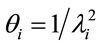 , i = 1, ···, n, and n is the number of days with daily hospitalizations above 28 (≥28) due to respiratory diseases in the period of 3621 days (from January 1, 1998 to November 30, 2007) in the Ribeirão Preto region. Observe that in (1) it was used a
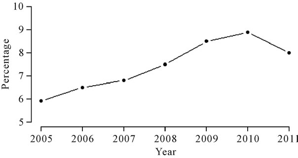
Figure 1. Percentage of yearly patient hospitalizations related to Chapter 10 of CID-10 in Ribeirão Preto.
Figure 2. Number of daily hospitalizations in the period from January 1, 1998 to November 30, 2007.
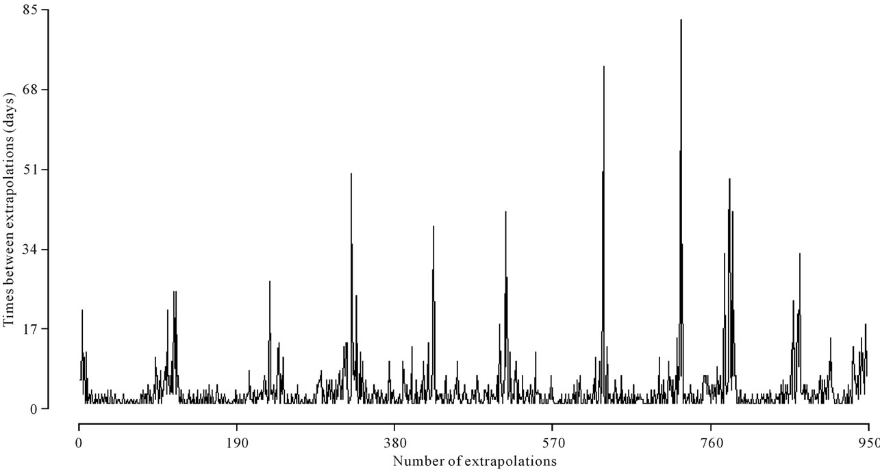
Figure 3. Times between threshold days in the period from January 1, 1998 to November 30, 2007.
reparametrized form of the exponential distribution.
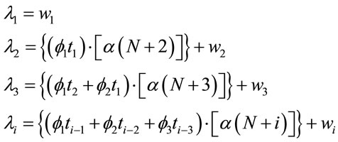
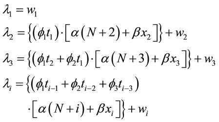
Different models can be considered for the hazard function ; as a first modeling, we assume the model,
 (2)
(2)
where ,
,  and
and ,
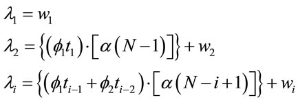
,  , for i = 3, 4, ···, n where wi is a non-observed random factor with an uniform distribution given by,
 (3)
(3)
where  denotes an uniform distribution. The parameters
![]() ,
, ![]() and
and  defined in (2) are assumed unknown. Let us denote the model defined by (1), (2) and (3) as “model 1”.
Observe that despite the independence assumption between the evaluated times (an arguable assumption) the ![]() and
and  terms given in (2), give an auto-regressive contribution of order 1 and 2, respectively, of the value of the time variable between over-hospitalizations in the hazard function of the exponential distribution with density (1).
Observe that in “Model 1” we are considering the term  in the modeling of the hazard function
 , i = 3, 4, ···, n, that is, we have a decreasing hazard in each extrapolation.
An alternative would be to assume the term  in place of the term
  which implies in increasing hazards
 , that is, decreasing mean times
![]() ; in this way, let us consider the “model 2” given by,
; in this way, let us consider the “model 2” given by,
 (4)
(4)
where 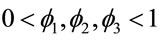 and
and ,
,  , for i = 4, 5, ···, n where wi is a non-observed random factor with an uniform distribution given by (3).
2.2. Modeling for Over-Hospitalizations Times and Field Burnings
The burning of biomass releases immediately in the atmosphere gases and particulate matter (PM), which consists most of fine and ultra-fine particles that are the ones most dangerous to the body, once these particles could enter the respiratory system starting an inflammatory process (see for example, Arbex et al. [4]).
Other elements that are released in the atmosphere by field burnings are the carbon dioxide, carbon monoxide, methane, non-methane hydrocarbons, nitric oxide and methylene chloride (see for example, Magalhães et al. [2]).
Following Baird [7] the particulate matter (PM), consisting of both fine and coarse particles, stay in the atmosphere by approximately 10 days. In this way, for the statistical modeling approach considering the field burnings, for each day with over-hospitalizations, we report the amount of field burnings that occurred in the last 10 days, for example, if the hospitalization number stayed above or equal to 28 in the day April, 27, we accumulate the amount of field burnings between the days April, 18 and April, 27.
To relate field burnings with over-hospitalization times it will be analysed the period March 1, 2005 to November 30, 2007, since the field burning data set presented many missing information before this period.
In Figure 4, we can observe the existing relationship between the over-hospitalizations and the accumulated number of field burnings in the 10 days before the occurrence of the event of interest.
To verify the possible association between cane fields burnings and times between over-hospitalization days due to respiratory diseases it was added to the model a “dummy” covariate X, given by xi = 0, if the number of field burnings in the last 10 days is < 11 and xi = 1 in other cases. This cut-off point was fixed based on the largest mean average observed between the over-hospitalization days. Therefore, when we assume the value 11 as a cut-off point, we find an average difference equals to 3.84 days between the groups <11 and ≥11, that is, it is the point that better differentiates the times between over-hospitalization days. In this way, we added the covariate X for the models in Section 2.1, that is,
 (5)
(5)
where ,
,  and
and , for i = 34, ···, n, where wi is a non-observed random factor with a uniform distribution given by (3). Denote the model defined by (1), (5) and (3) as “model 3”.
The next proposed model for the hazard function is given by,
 (6)
(6)
where 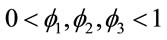 and
and ,
,  , for i = 4, 5, ···, n where wi is a non-observed random factor with an uniform distribution given by (3). Denote this model as “model 4”.
3. A Bayesian Analysis
For the different models introduced in Sections 2.1 and 2.2, we assume prior independence among the parameters of the models [8].
Samples of the joint posterior distributions of interest considering each proposed model are simulated using standard existing MCMC (Markov Chain Monte Carlo) methods. We use the WinBUGS software [9] which only requires the specification of the distribution for the data and the prior distributions for the parameters of each proposed model.
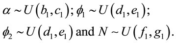
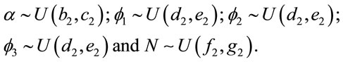
Different prior distributions were specified for each case. Considering “model 1”, we assumed the following prior distributions for the random quantities![]() ,
, ![]() ,
,  and N:
Figure 4. Times between over-hospitalization days and number of field burnings, in the period March 1, 2005 to November 30, 2007.
 (7)
(7)
The hyperparameters b1, c1, d1, e1, f1 and g1 are assumed to be known. In the same way, we consider the prior distributions for parameters of “model 2”.
It is important to point out that the choice of the hyperparameter values of the prior distributions (7) could be based on prior expert opinions or using empirical Bayesian methods [10]. In some cases the values of the hyperparameters were chosen in a way to have approximately non-informative priors.
Considering the “model 2”, the following prior distributions are assumed:
 (8)
(8)
Considering models 3 and 4, we assumed the same priors considered for models 1 e 2, respectively.
To discriminate for the best model, we have used standard existing Bayesian methods; one of these techniques is given by the DIC (Deviance Information Criterion) [11] where smaller values of DIC, indicate better fit of the data for the assumed model. Another possibility to check for the best fit is to compare the estimated means  for each model, where
  is the Monte Carlo estimate of the posterior mean for
  based on the simulated Gibbs samples, with the observed times ti. In this way, we can compare the difference sums
 , i = 1, ···, n for each assumed model.
4. Results
For the simulation of the Gibbs samples, we first simulated 3000 samples, discarded to eliminate the effect of the initial values in the simulation algorithm (“burn-insample”). After this burn-in period, another 125,000 samples were generated, from which every 25th sample was taken, which totalizes a final sample of size 5000 to be used to get the posterior summaries of interest. This step of size 25 was chosen to have approximately uncorrelated final samples. For all cases it was simulated three independent chains for each assumed model; the convergence of the Gibbs sampling algorithm was monitored using standard existing graphical methods, as the traceplots of the simulated samples and a convergence index introduced by Gelman and Rubin [12]. All simulation process was obtained using the WinBUGS software.
In Table 1, we have the prior distributions assumed for models 1, 2, 3 and 4. For all these priors we have approximately no prior information. Discrimination of the proposed models was made using DIC and the values for the sums of the estimated means and the observed values using the following equation,
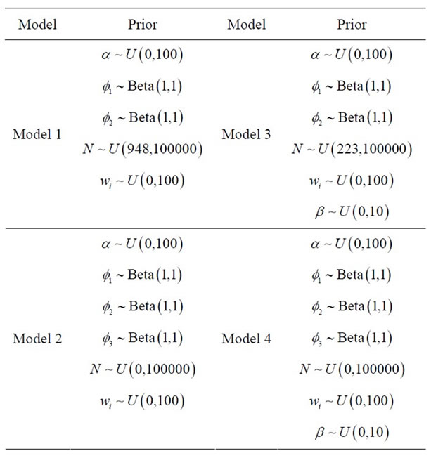
Table 1. Prior distributions for the parameters of the proposed models.
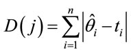 (9)
(9)
where j indexes the model.
In Table 2, we have the Monte Carlo estimates for the posterior means and posterior standard deviations for the parameters of models 1, 2, 3 and 4; we also have the Monte Carlo estimates for DIC given automatically by the software WinBUGS and the values for the sums of differences given by formula (9).
From the results of Table 2, we observe that the best fitted model using DIC criterium is the “model 3”; using the sums of differences given by formula (9), “model 1” is the best fitted model (smallest value for  for j = 1).
From these considerations on the fit of the models, we present some interpretations of the obtained results (see, Table 2) considering models 1 and 3. These interpretations are easily extended to models 2 and 4, respectively.
First of all, let us take “model 1”. We observe that all parameters are significative, that is the associated 95% credible intervals do not includes the zero value. The same was observed for the other models.
The parameter![]() , is directly related to the hazard function λ of the exponential distribution, that is, inversely related to the mean θ of the times of over-hospitalizations; in other words: larger values for
, is directly related to the hazard function λ of the exponential distribution, that is, inversely related to the mean θ of the times of over-hospitalizations; in other words: larger values for ![]() implies in smaller values for θ.
implies in smaller values for θ.
The parameter N also has the same effect of α. The parameters ![]() and
and  represent a contribution of the previous times on the current estimated time. The parameter
 ![]() represents the effect of the previous time on
represents the effect of the previous time on
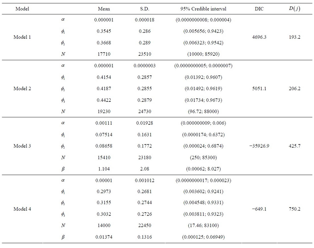
Table 2. Posterior summaries for models 1, 2, 3 and 4.
the hazard, while , represents an auto-regressive effect of order 2, that is, it is dependent of the penultimate previous time. In models 2 and 4 there is an additional parameter
 , that gives a contribution of an auto-regressive effect of order 3. As the mean time is estimated by
 , larger values of the auto-regressive parameters, smaller the estimated mean times.
Finally, we interpret the parameter β, where in the same way as the other parameters, as larger its estimative, smaller is the over-hospitalization times. As their estimatives are larger than zero and their respective 95% credible intervals do not include the zero value, we can say that when the accumulated number of field burnings is >10, the effect in which β affects the estimated time implies that this value decreases; this result is totally in agreement with many published results, that is, the field burnings have a harmful effect on the respiratory systems of the population.
In all cases, it was observed convergence of the simulation MCMC algorithm used to generate samples of the joint posterior distribution of interest.
5. Concluding Remarks
Many studies given in literature confirm the existence of an association between field burnings and an increasing in patient hospitalizations due to respiratory diseases, especially in newly borns and elderly persons [13].
However studies on the times between over-hospitalizations are not very well studied in the literature. In this paper, we introduce new modeling approaches for these times related to respiratory diseases in the Ribeirão Preto region, with the inclusion of a covariate denoted by X associated to the presence of field burnings.
Under a Bayesian approach, we get the posterior summaries for the parameters of interest, using MCMC methods and the free available WinBUGS software. We observe that models not in presence of the covariate field burnings show more accurate estimates, but, with the inclusion of this covariate the models showed a great improvement in terms of quality, observed in the values of the estimated values for DIC.
The fitted models in presence of the covariate field burnings X give evidences that the sugar cane field burnings have a significative effect on the times of over hospitalizations due to respiratory diseases, that is, the presence of 11 or more field burnings in the previous 10 days before an over number of hospitalizations implies in smaller time between over hospitalizations by respiratory diseases in the Ribeirão Preto region. This result is important to show that laws and regulamentations for sugar cane field burnings should be maintained and monitored by the health government authorities since sugar cane field burnings could increase the number of hospitalizations due to respiratory diseases.
Although autoregressive factors do not indicate a great effect on the estimated means between over hospitalizations, these factors are important as part of the models introduced in this paper, since they are important to minimize the autocorrelation among the residuals.
These new models introduced in Section 2 present a random effect or non-observed variable, which gives a great flexibility of fit and also permit to estimate in an easily way, the presence of multiple change points, since a great part of the variability is explained by the random effects.
6. Acknowledgements
The authors are grateful to the Brazilian institutions CAPES and CNPq for the grants to develop this research.
REFERENCES
- Brazil, Ministério da Saúde. Secretaria Executiva. DATASUS. Informações de Saúde. Morbidade Hospitalar do SUS por local de internação. http://tabnet.datasus.gov.br/cgi/deftohtm.exe?sih/cnv/nisp.def
- D. Magalhães, R. E. Bruns and P. C. Vasconcellos, “Polycyclic Aromatic Hydrocarbons as Tracers of Burning Cane Sugar: A Statistical Approach,” Química Nova, Vol. 30, No. 3, 2007, pp. 577-588. doi:10.1590/S0100-40422007000300014
- F. S. Lopes and H. Ribeiro, “Mapping of Hospitalizations for Respiratory Problems and Possible Associations to Human Exposure to Products of Straw Burning of Sugar Cane in São Paulo,” Brazilian Journal of Epidemiology, Vol. 9, No. 2, 2006, pp. 215-225.
- M. A. Arbex, J. E. D. Cançado, L. A. A. Pereira, A. L. F. Braga and P. H. N. Saldiva, “Biomass Burning and Its Effects on Health,” Brazilian Journal of Pulmonology, Vol. 30, No. 2, 2004, pp. 158-175.
- L. C. Martins, M. R. D. O. Latorre, M. R. A. Cardoso, F. L. T. Gonçalves, P. H. N. Saldiva and A. L. F. Braga, “Air Pollution and Emergency Room Visits for Pneumonia and Influenza in Sao Paulo, Brasil,” Revista de Saúde Pública, Vol. 36, No. 1, 2002, pp. 88-94. doi:10.1590/S0034-89102002000100014
- Banco de Dados Queimadas (BDQUEIMADAS). http://www.dpi.inpe.br/proarco/bdqueimadas/
- C. Baird, “Environmental Chemistry,” 2nd Edition, W.H. Freeman and Company, New York, 1999.
- J. M. Bernardo and A. F. M. Smith, “Bayesian Theory,” Wiley, Chichester, 1994. doi:10.1002/9780470316870
- D.J. Lunn, A. Thomas, N. Best and D. Spiegelhalter, “WinBUGS—A Bayesian Modelling Framework: Concepts, Structure, and Extensibility,” Statistics and Computing, Vol. 10, No. 4, 2000, pp. 325-337. doi:10.1023/A:1008929526011
- B. P. Carlin and T. A. Louis, “Bayes and Empirical Bayes Methods for Data Analysis,” 2nd Edition, Chapman and Hall, Boca Raton, 2000. doi:10.1201/9781420057669
- D. J. Spiegelhalter, N. G. Best, B. P. Carlin and A. Van Der Linde, “Bayesian Measures of Model Complexity and Fit,” Journal of the Royal Statistical Society, Series B, Vol. 64, No. 4, 2002, pp. 583-639. doi:10.1111/1467-9868.00353
- A. Gelman and D. R. Rubin, “Inference from Iterative Simulation Using Multiple Sequences,” Statistical Science, Vol. 7, No. 4, 1992, pp. 457-472. doi:10.1214/ss/1177011136
- D. Rigueira, P. A. Andre and D. M. T. Zanetta, “Sugar Cane Burning Pollution and Respiratory Symptoms in Schoolchildren in Monte Aprazível, Southeastern Brazil,” Revista de Saúde Pública, Vol. 45, No. 5, 2011, pp. 878- 886.