International Journal of Astronomy and Astrophysics
Vol.4 No.1(2014), Article ID:43663,29 pages DOI:10.4236/ijaa.2014.41018
Simulations of Colliding Uniform Density H2 Clouds
Guillermo Arreaga-García1, Jaime Klapp2,3, Julio Saucedo Morales1
1Departamento de Investigación en Física, Universidad de Sonora, Hermosillo, Mexico
2Instituto Nacional de Investigaciones Nucleares, Ocoyoacac, Mexico
3Departamento de Matemáticas, Cinvestav del Instituto Politécnico Nacional, México D.F., Mexico
Email: garreaga@cifus.uson.mx, jaime.klapp@inin.gob.mx, jsaucedo@cifus.uson.mx
Copyright © 2014 by authors and Scientific Research Publishing Inc.
This work is licensed under the Creative Commons Attribution International License (CC BY).
http://creativecommons.org/licenses/by/4.0/


Received 18 December 2013; revised 18 January 2014; accepted 25 January 2014
ABSTRACT
In this paper we present a set of numerical simulations designed to study the interaction process of HII molecular clouds. For the initial conditions we assume head-on and oblique collisions of binary identical clouds placed adjacent to one another, with their surfaces just in contact. The colliding initial clouds are uniform density molecular gas spheres with rigid body rotation. The cloud initial conditions are chosen to favor its gravitational collapse as an isolated system. To study the effect of the self-gravity of the cloud in the collision process, we consider several models in which the approaching speed of the colliding clouds increases from zero up to several times the initial sound speed of the barotropic gas. We present the outcome of these collision models for several values of the impact parameter b, which depends on the initial radius of the cloud. We have explored the parameter space of the approaching velocity Vapp of the colliding clouds for configurations that may result in seeds for the formation of more complex systems. Such systems are expected to include filaments and gas clumps, where the star formation process is still possible despite the occurrence of the collision. We show hereby that collisions may have a major and favorable influence on the star formation process.
Keywords:Star Formation; Cloud Collisions; Protostellar; Binaries

1. Introduction
Protostellar cloud collisions are expected to occur in a great variety of astrophysical phenomena, for example, as a consequence of collisions between gas-rich galaxies; or due to the presence of strong tidal forces within a single giant cloud. For instance, [1] identified mechanisms they suggested could initiate the formation of agglomerations of matter within the cloud, due to the expansion of regions leading to a compression in other regions of the same cloud. He presented observational evidence of gas compression at the interface of two colliding molecular clouds, and proposed that collisions may be an alternative mechanism to explain the formation of massive stars in galaxies. Indeed, collisions between neutral molecular clouds are frequently mentioned as a possible mechanism for initiating the star formation process. For instance, based on observed carbon molecular lines, [2] suggested that the formation of the stars in the IRAS04000 + 5052 cluster was induced by the collision of two molecular clouds.
The theoretical study of collisions has a long history. It was started in the early 80 s, but even nowadays the academic interest in astrophysical collisions has never fallen off completely, see for instance [3] [4] .
In the old numerical simulations of colliding gas clouds that were done with particle based codes, the clouds partially penetrated each other; and in the case of collisions with high Mach numbers, they passed completely one to another, see [5] . These non-physical results were the consequence of the neglect of artificial viscosity that was later used by [6] .
In simulations based on grid techniques, there were also important limitations, for example, those considering only two spatial dimensions or neglecting self-gravity. In spite of this, the complexity of the phenomenon was uncovered many years ago. For instance, [7] studied head-on collisions with several two clouds combinations, in which one of them represented a giant molecular cloud, and the second one was smaller and denser than the former. They also considered several cases according to the internal density structure of the clouds: some were uniform while others clumpy. In their two dimensional hydrodynamical calculations, the effect of the self-gravity of the gas was unfortunately not taken into account.
Besides, [8] performed two dimensional collision simulations between atomic hydrogen clouds using the AMR (Adaptive Mesh Refinement) numerical technique. In their hydrodynamic equations, they included heating and cooling functions as well as a magnetic pressure term. They considered homogeneous clouds with cylindrical symmetry and surface perturbations, and showed that a filament forms at the interface of the clouds and that the gas flow outwards from the edge of the filament. They estimated that a numerical simulation based on particles with a similar resolution should include at least one million particles. Unfortunately, again their simulations did not include self gravity.
Additionally, [9] also considered collisions between giant spherical clouds within the framework of the Smoothed Particle Hydrodynamics (SPH) Lagrangian technique. The mass of each cloud was 2222M⊙ with a radius of 10 pc. Their collision models with clouds at a temperature of 20 K and with an approaching speed of 10 km∙s−1 produced fragments with a size of 0.1 pc and with a peak density number of 104 cm−3. The conclusion of their calculation was that cloud collisions certainly stimulate the formation of clumpy structures. A drawback of this study is that the authors only used 4096 particles to model such a huge cloud.
There are non-spherical collision models reported in the literature as well, for instance [10] considered two identical, parallel gas slabs, semi-infinite in extent so that each slab could be considered two dimensional, in such a way that the collision takes place in only one spatial dimension.
Although the papers mentioned above are only a representative sample of the vast amount of existing literature, in view of them, we believe it is timely to devote this paper to make new numerical simulations of the collision process, taking advantage of both new capabilities of modern computers and improved numerical techniques.
We now present numerical high resolution three-dimensional (3D) hydrodynamical simulations of spherical cloud collisions, including the self-gravity of the gas. As mentioned earlier, we restrict ourselves to considering only binary collisions between identical clouds.
Our main objective in this paper is to explore the parameter space of the collision models; we have proposed several approaching velocities, simply as sample values chosen only on the basis of the different outcomes that each simulation produces. We also emphasize that along this project we are always interested in studying the effects of the collision on a cloud which is already collapsing. Another subject deserving further study, is the case of clouds starting from hydrodynamical equilibrium.
This was already considered by [4] [11] , who simulated cloud collisions between two clouds initially in hydrodynamical equilibrium (since each cloud was modeled as Bonnor-Ebert sphere). Collisions between dissimilar clouds has also considered by [12] . An important result of our simulations, is that we have explored the possible approaching velocities of the colliding clouds (for an initial cloud with well defined physical characteristics, see Section 2). Because of this, we now know the range of approaching velocities that allow an initial binary colliding clouds system to remain as a binary system capable of undergoing further gravitational collapse and eventually produce a multiple protostellar system. It is in this sense that our results have to be compared with those of [13] , that obtained that it is more likely that a colliding system will in general result in disruption and dispersal of the cloud involved with no chance of forming proto stars.
It must be emphasized that this work hereby devoted to study collisions with clouds with a clear initial tendency to a gravitational collapse prior to collision, has enabled us to uncover subtle collision effects about the formation and fragmentation of the collapsing clumps. To have observed these effects have made an important difference in the results derived from the simulations when we compare with those results reported by [4] [11] [12] .
Besides, during the phase that comes after the collision before the density reaches the critical density ρ ~ 10−18 gr∙cm−3, shearing and Kelvin-Helmholtz instabilities are observed. Fragmentation has been observed in somefilaments, which is a direct consequence of the occurrence of the collision. The integral properties of the resulting gas clumps are calculated with the purpose of estimating if they are likely to collapse, virialize or disperse. The initial conditions for the isolated cloud are such that it will collapse in the absence of a collision as its thermal and rotational energy ratios with respect to the gravitational energy, have been chosen to have initially the numerical values α0 = 0.26 and β0 = 0.16, respectively. However, when we consider the translational kinetic energy that comes from the approaching velocity Vapp of the clouds, the collision system is unbound for Vapp greater than about Mach three. As a result of the collision process a large fraction of the translational kinetic energy is transformed into heat that is radiated away because the clouds and the shock front that forms in the interphase between the clouds are isothermal. This produces are duction of the global value of α + β for all models. For the head-on models we found that they all get a final configuration near equilibrium even for very high Vapp. This is not the case for the oblique models, which have a final value near equilibrium for Vapp less than about Mach three and all b values. The final α + β values get away from equilibrium for Vapp greater than Mach eight and high b values. Hence we only get very high dissipation, and thus the possibility of fragmentation for initially unbound systems for head-on or near head-on collisions.
The observation that collisions favor molecular cloud fragmentation is a very important result in the area of star formation, because each dense gas knot formed along the filament in the central core of the colliding cloud, could eventually form a proto-star.
The outline of the paper is as follows. In Section 2 we describe the characteristics of the particle distribution that represents the initial cloud, which will be involved in all the subsequent collisions. In Section 3 we show the geometry of the collision models and the parameter values chosen for the Gadget2 code. In Section 4, we describe the most important features of the time evolution of our simulations by means of two-dimensional (2D) isodensity plots, despite the fact that the collision events are fully 3D. In Section 5 we discuss the relevance of our results in view of those reported by previous works and finally we make some concluding remarks.
2. The Initial Cloud
We consider a spherical cloud with radius R0 = 3.0138 × 1018 cm = 0.97 pc = 2.0038 × 10⁵ AU and mass M0 = 2.21M⊙. The average density of this cloud is ρ0 = 1.3024 × 10⁻²¹ gr/cm3, from which we can estimate the time required by a test particle to reach the center of the cloud from the outermost regions, known as the free fall time of the cloud and given by
 (1)
(1)
Our initial cloud can be considered as a typical prestellar cloud, though of a very small size such that it can be called a clump according to [14] . It is relatively easy to observe these small clouds as isolated systems in low mass star forming regions such as Taurus [15] . If these clouds have also existed within more dense cloud environments such as the Orioncluster, they would have had multiple dynamical encounters. In the collision events more frequently observed, the involved clouds are very likely to be typical giant molecular clouds with radius ~ 40 pc and mass ~ 105 M⊙.
We have set five million SPH particles to generate the initial cloud by a traditional Monte Carlo scheme, in which the particles are randomly located in the volume space. Let u, v and w be random uniform variables taking real values within the interval [0,1]; then according to the fundamental probability conservation law for a system with spherical symmetry, we have that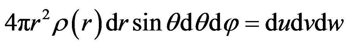 . By means of integration we obtain that the spherical coordinates
  of the particles are related to the uniform random variables by the following equations:
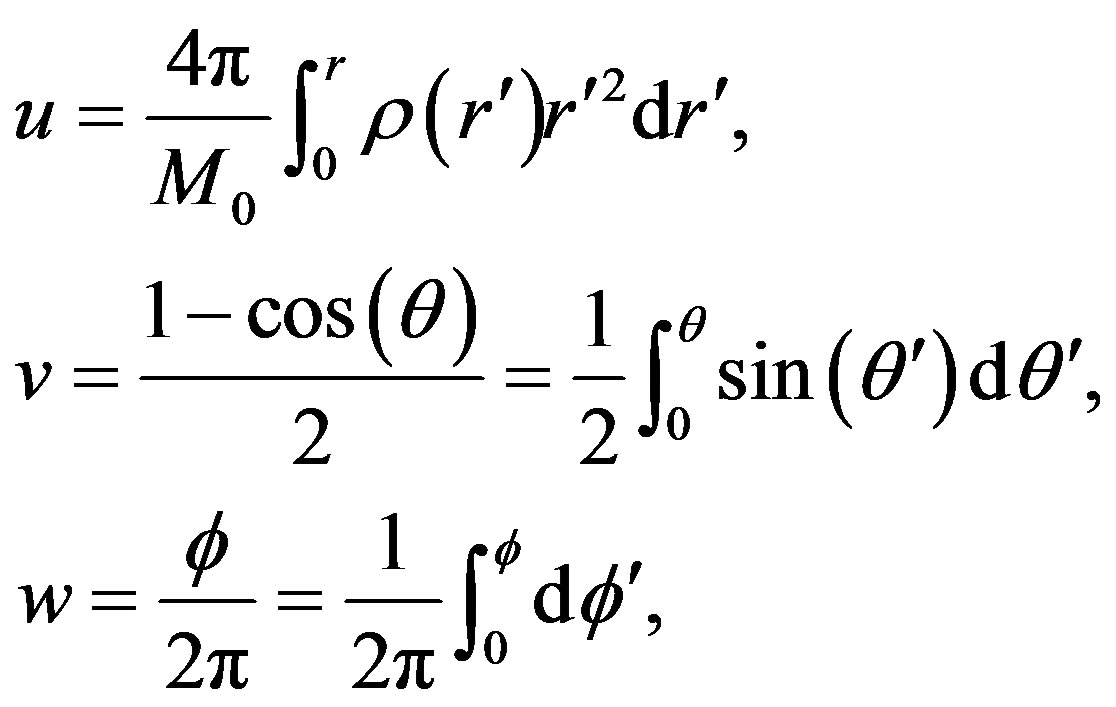 (2)
(2)
where M0 is the total mass contained in the cloud of radius R0; it must be noticed that the first relation should be numerically integrated to obtain r once that u has taken an allowed uniform random value. The mathematical function f(r) in which we are interested to model the cloud’s radial distribution of matter was first introduced by [16] , and later on studied by [17] as a building block of an analytical model to study the collapse of clouds. This radial density function is given by:
 , (3)
, (3)
where ρc, Rc and  are three free parameters that fix the shape of the radial density profile.
As it was mentioned by [16] , the main characteristic of this Plummer-like density function is its radial behavior: constant at first and then rapidly falling off with radius. Due to the density behavior, this mathematical model captures quite well the observed fact that prestellar clouds are mainly formed by a strongly centrally condensed low mass core, which is surrounded by a gas envelope steeply declining in density, see [15] .
The Plummer parameters are Rc = 3.0 × 1018 cm and ρc = 1.3025 × 10⁻²¹ gr∙cm−3. The initial radius R0 is slightly larger than Rc, because for this paper we are mainly interested in studying the collision of uniform density clouds, see Figure 1. The cutting density ρc is very near the average density ρ0. In an article to come, we will study collisions between centrally condensed clouds, in which Rc < R0. This future study promise to be interesting, as [18] [19] have already shown that the extension of the envelope with respect to the core in a centrally condensed cloud, is also an important dynamical factor playing a crucial role in the fate of the cloud’s collapse.
Additionally, we consider that the cloud is in counterclockwise rigid body rotation around the Z axis; therefore the initial velocity of the i-th SPH particle is given according to , where Ω0 is the constant magnitude of the initial angular velocity. For the cloud considered in this paper, the initial sound speed and angular velocity have the following values:
 (4)
(4)
As it is quite common in the literature of gravitational cloud collapse [20] [21] , the dynamical properties of the initial distribution of particles modeling the cloud are usually characterized by means of the thermal and rotational energy ratios with respect to the gravitational energy, denoted by α and β, respectively. The ρ0 and Ω0 values have been calculated for the energy ratios to initially have the following numerical values:
 (5)
(5)
We recall that these selected values of α and β are known to favor the occurrence of collapse in the cloud.
As done in our previous papers, we also implement a density perturbation on the initial particle distribution, such that at the end of the evolution of the cloud as an isolated system, it might result in the formation of binary systems. This perturbation is applied to the mass of each particle mi according to:
 (6)
(6)
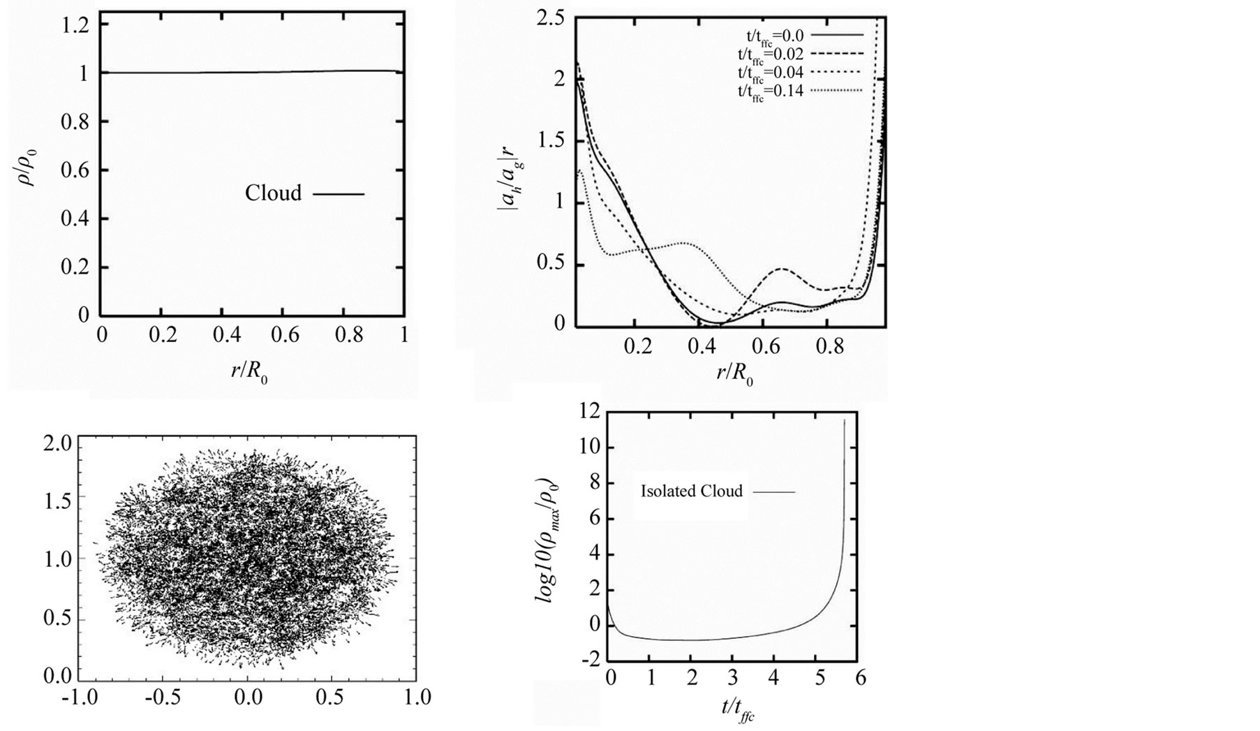
Figure 1. Upper left panel: Radial density profile for the distribution of SPH particles modeling the initial uniform cloud, as measured from the first Gadget2 snapshot. Upper right panel: Ratio of the hydrodynamical (due to the pressure gradient only) to the gravitational acceleration for several times of the first stage of the cloud’s evolution. Lower left panel: Velocity field of an XZ view of a collision scenario where the velocity of cloud’s particles is seen to point outwards during the initial evolution stage. Lower right panel: The time evolution of the peak density obtained for the collapse of the cloud as an isolated system.
where m0 is the unperturbed mass of the simulation particle, the perturbation amplitude is set to a = 0.1 and the mode is fixed to m = 2. We have found that this mass perturbation is almost irrelevant in the scenario of the cloud collision models.
The characteristics and physical properties of the clouds expressed in Equations (5) and (6) are quite common and we refer the reader to [20] [21] for reviews of the most important results of collapse calculations which have given place to great conceptual advances in the state of the art.
Let us now say something about the way in which we account for the thermodynamics of the gas. Most authors have used an ideal equation of state. As the observed star forming regions basically consist of molecular hydrogen clouds at 10 K with an average density of 1 × 10⁻²⁰ gr∙cm−3, the ideal equation of state is a good approximation. However, once that gravity has produced a substantial contraction of the cloud, the gas begins to heat. In order to take into account this increase in temperature, we use the barotropic equation of state proposed by [22] . Thus in this paper we carry out all our simulations using the following equation of state:
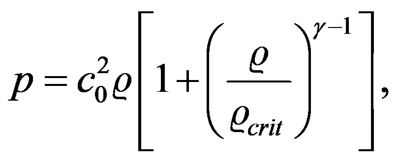 (7)
(7)
where for the molecular hydrogen gas the ratio of specificheats  because we only consider translational degrees of freedom of the hydrogen molecule. For the critical density we consider only one single value of
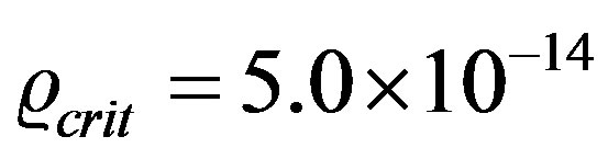 gr∙cm−3.
However, a word of warning should be made. By comparing the results of our previous works in [23] [24] with those of [25] for the collapse of an isolated and rigidly rotating cloud with a uniform density profile, we have concluded the barotropic equation of state in general behaves quite well and that it captures all the essential thermo dynamical phases of the collapse. But this does not mean that the same comparison would always be correct for more complex initial conditions or for collision models as those we are considering in this paper.
Despite these facts and that we know that it is indispensable to include all the detailed physics of the thermal transition in order to achieve the correct results, be it in a collision or not, we carry out the present simulations with the barotropic approximation, because we know that there are other computational and physical factors that could have a stronger influence on the outcome of a simulation.
The collision clouds considered for this work have approaching velocities of up to about thirty times the sound speed, see Section 3 and Table 1. For these high velocities a shock is formed in the interface between the clouds and the artificial viscosity used for the calculations transform kinetic into thermal energy that increases the gas temperature. However, as we will now show, the cooling time  is both much shorter than the local sound crossing time, and the free fall time, hence the isothermal condition can be used for the shock region.
For an initial density of the clouds of  gr∙cm−3, its particle number density is
  cm−3, where mp is the proton mass and μ the mean molecular weight of the gas, which we take to be 2.4. For a strong adiabatic shock, from the Rankine-Hugoniot jump condition, the density in the thin dissipative region is about four times the pre-shock density, and so we expect the post-shock number density to be about
 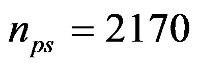 cm−3.
cm−3.
We can calculate the cooling time from the expression [26]
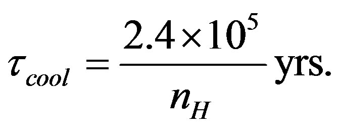 (8)
(8)
Using our estimate for the post shock region we obtain that . On the other hand, for our clouds the local sound crossing time
  and the free fall time
 . We can then assume that the shock remains isothermal.
3. Collision Models and Computational Considerations
In this paper we use the Gadget 2 code which implements the SPH technique. We use five million simulation particles to model each colliding cloud, as we explain below.
3.1. The Collision Geometry
The simulations considered in this paper include both head-on and oblique collisions, see Figure 2. For the head-oncollisions, the initial position in rectangular coordinates of the center of mass (CM) of each of the colliding clouds is located at  and
and , respectively. We recall the reader that R0 is the initial radius of the cloud.
The average velocity of the center of mass of the clouds points along the Y axis and are  and
and . We define the approaching speed Vapp (with respect to the center of mass of the collid

Table 1. The collision models.

Figure 2. The initial geometry of the colliding clouds for the head-on collision (left panel), and for the oblique collisions with a positive impact parameter b (right panel).
ing binary system) of the clouds by means of Vapp = 2 Vave.
For the oblique collision case, the colliding clouds are initially displaced (with an impact parameter b along the X-axis) transversely to the collision symmetry axis (the Y-axis). For these cases, the center of mass of the clouds are initially placed at the coordinates  and
and , see Figure 2. The approaching velocity is defined in the same way as was done for the head-on collision case.
To consider a significant sample of models, we choose severalimpact parameters and approaching velocities. For instance, the impact parameter takes the values b = 0, R0/2, R0 and 2R0. It should be noticed that this range of values is well motivated physically, as it follows from an statistical cloud collision study in the context of interacting galaxies [27] .
3.2. The Collision Approaching Velocity
With the purpose of studying the influence of the self-gravity of the cloud in the outcome of the collisions, we define several models in which we change the cloud’s displacement speed Vave. Therefore, according to the collision model under consideration, each colliding cloud can individually reach different stages of gravitational collapse before the collision takes place.
It has been known since the first molecular line studies that most molecular clouds are observed to have a hierarchical structure, which consist of small gas condensations in supersonic random motion embedded in a larger and more diffuse parent cloud. According with the classification scheme of [14] , such small gas clumps are observed to have a size between 0.3 and 3 pc and a velocity in the 0.3 - 2 km∙s−1 range. For instance, let usmention two cloud examples reported by [28] : the cloud OMC1within the Orion Complex, which has a velocity dispersion of 2.5 km∙s−1, size of 1.2 pc and a mass of 1000M⊙; the clouds B7 and B19 observed in the Taurus complex have a velocity dispersion of 0.9 km∙s−1, a similar size of 1.0pc, but with a mass of 140M⊙, much smaller than for the OMC1 cloud.
These data for molecular cloud condensations have common features with the clouds modeled in this manuscript. Bergin [14] also reported that the typical sound speed for this kind of cloud (with a temperature around 10 K), is approximately $c0 = 0.2 km∙s−1. Then, for such random movements the ratio v/c0 of the velocity of the cloud to the sound speed, would be in the range Mach v/c0 = (0.3/0.2 - 2/0.2) = (0.15 - 10). Now, if we want to consider a collision between two of this kind of gas clumps, then the approaching velocity (also known as the relative or impact velocity of the clouds) of the colliding clouds will at least be 2v/c0, which gives us an approaching velocity Vapp in the range Mach (0.30 - 20).
In order to be consistent with the observational data we have just described, the approaching velocity formost of our models has been chosen in the range Mach (0 - 10). Besides, we have included model HO-5 with an approaching velocity of Mach 30 just for the sake of comparison with [4] that modeled cloud collisions with Mach 25 and 35 and those of [29] that also modeled cloud collisions with velocities in the range Mach (25 - 40).
In Table 1 we summarize all the collision models considered in this paper. The entries of the data in Table 1 are as follows. Column one shows the label chosen to identify the model. Column two indicates the impact parameter b of the collision models in terms of R0; it should be noticed the appearance of a sign before the magnitude of b, whose meaning will be explained in detail below in Section 4.4, but in advance we say that it is related to the orientation of the colliding clouds along the X-axis. Column three indicates the approaching velocity of the colliding clouds, expressed in terms of the initial sound speed of the cloud, whose numerical value is given in Equation (4). Columns four and five show the peak density and maximum evolution time reached in our runs following the colliding process. We recall that we normalize density and time with the average density  gr∙cm−3, and with the free fall time
  Myr, respectively.
For each individual cloud α = 0.26055 and β = 0.16143, see Equation (5), which gives that α + β = 0.42693. For the initial collision systems we show in columns six, seven and eight the global values of α, β and α + β and in columns nine, ten and eleven the same quantities for the last computed model for each of the initial configurations. The values for the last six columns are calculated for the global collision system and includes the kinetic translational energy that after the collisions contribute to the α and β values of the resulting system. From the column eight of Table 1 we notice that only models HO-1, M1, M2 and M4 are bound, that is only for systems with Vapp/c0 less than about three. In Table 2 we sum up the main result of the collision models.
3.3. The Evolution Code
We carry out the time evolution of the initial distribution of particles with the fully parallel Gadget2 code, which is described in detail by [30] . Gadget2 is based on the tree-PM method for computing the gravitational forces and on the standard SPH method for solving the Euler equations of hydrodynamics.
Gadget2 incorporates the following standard features: (i) each particle i has its own smoothing length hi; (ii) the particles are also allowed to have individual gravitational softening lengths εi, whose values are adjusted such that for every time step εihi is of order unity. Gadget2 fixes the value of εi for each time-step using the minimum value of the smoothing length of all particles, that is, if hmin = min(hi) for i = 1, 2... N, then εi = hmin.
The Gadget2 code has an implementation of a Monaghan-Balsara form for the artificial viscosity [31] [32] . The strength of the viscosity is regulated by setting the parameter  and
and , see Equation (14) in [30] . We have fixed the Courant factor to 0.1.
3.4. Resolution
According to [33] , the resolution requirement for avoiding the growth of numerical instabilities is expressed in terms of the Jeans wavelength , which is given by
 (9)
(9)
Table 2. The main outcome of the collision models.
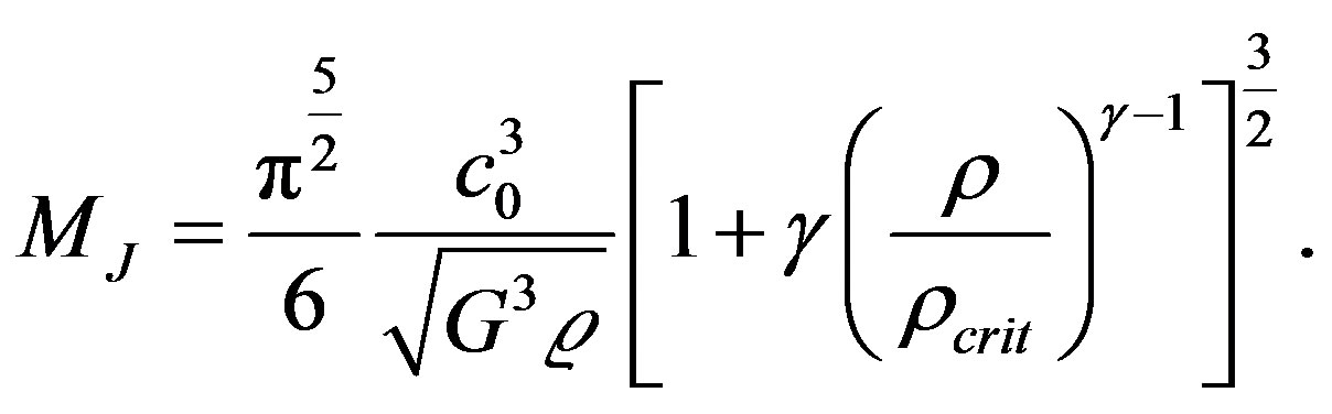
where G is Newton’s universal gravitation constant, c is the instantaneous sound speed and ρ is the local density. To obtain a more useful form for a particle based code, the Jeans wavelength λJ is written in terms of the spherical Jeans mass MJ, which is defined by
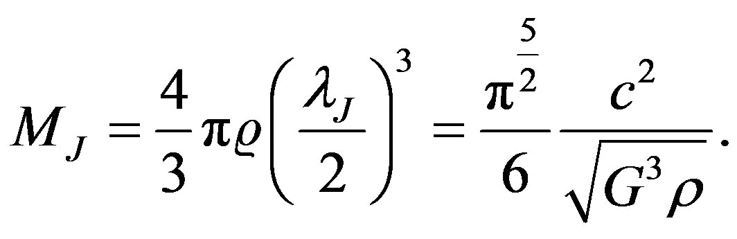 (10)
(10)
Nowadays it is well known that the Jeans requirement  (where l is a characteristic length scale of the grid for a mesh based code) is a necessary condition to avoid the occurrence of artificial fragmentation. For particle based codes, [34] showed that there is also a mass limit resolution criterion which needs to be fulfilled besides that of [33] . They showed that an SPH code produces correct results involving self-gravity as long as the minimum resolvable mass is always less than the Jeans mass MJ.
If we now approximate the instantaneous sound speed by , then according to Equation (7), we have
 (11)
(11)
Following [34] , the smallest mass that an SPH calculation can resolve is 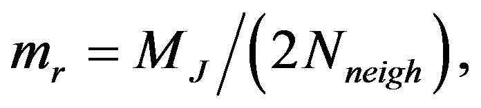 where Nneigh is the number of neighboring particles included in the SPH kernel. For our collision models to comply with the Jeans requirement, the mass particle mp must be such that mp/mr < 1.
The mass of the simulation particles is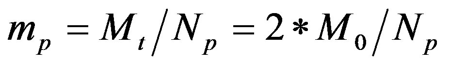 , where Mt is the total mass contained in the simulation box; the total number of particles Np is 10 million for all the models in this paper.
To verify that the Jeans stability condition is satisfied we will use the collision model HO-1, which is the one that reached the highest maximum density of all models, see Table 1. For this model we followed its collapse until a peak density of  gr∙cm−3. The average particle mass (after the mass perturbation given by Equation (6)) is
 .
.
For all models our assumed initial sound speed is given by Equation (4), and hence from Equation (11) the minimum Jeans mass for model HO-1 is given by , from which we obtain
  Thus, for model HO-1 we obtain the ratio
 , and the Jeans resolution requirement is quite easily satisfied.
For the rest of the collision models, the minimum Jeans mass is expected to be greater than for model HO-1 because their maximum density is less than for model HO-1. It is then clear that for all models the Jeans length criterion is satisfied as well.
4. Results
In order to show the main results of our simulations, we present iso-density plots for a slice of matter parallel to the XY plane. The procedure to illustrate the results of these 3D phenomena with 2Diso-density plots is as follows. We first locate the SPH particle with maximum density in the entire volume space of a simulation. The z-coordinate of that particle, say zmax, determines the height of the thin slice of material. The width of the slice is determined such that about 10,000 SPH particles enter into the slice, which is centered around the zmax coordinate. Once the SPH particles defining the slice have been selected, we set a color scale related to the iso-density curves: yellow colors indicate areas with higher densities, whereas blue those with lower densities and green and orange correspond to intermediate density regions. It should be noted that there is no relation between the density colors associated with different panels even in the same plot.
At the bottom of each iso-density panel, we include two numerical values to illustrate the different stages of the evolution process: the left value is the peak density ρ(t) at time t; and the right one the actual time t normalized with one of the two free fall times:  for the cloud and
  for the collision, as we explain below.
In fact, there is a further time scale that can be defined for the collision system, which is expected to be slower than for the isolated cloud because the spatial extension of the new system has doubled, and its average density is smaller than , and therefore its associated
  must be longer than
 . The new time scale is given by
 (12)
(12)
It should be clear that the times given in Equations (1) and (12) are only time estimates and are useful just as normalizing factors for our evolution plots.
The evolution of the uniform density cloud model has been reproduced by many groups worldwide using different codes based both on grids and particles, see for instance [20] [21] and references there in. We also successfully reproduced the uniform model results in [23] and [24] , from which we established there liability of our calculations for evolving the cloud with the Gadget2 code, as we followed the collapse process until peak densities of the order of  gr∙cm−3. Now, in this paper we use the same Gadget2 code to evolve the initial conditions for a bigger but still rotating cloud and to follow the process of the collisions as well.
4.1. The Collapse of the Initial Cloud
We describe in this Section the temporal evolution of the initial cloud as an isolated system which evolves under the influence of its own gravitational force. Numerical simulations performed so far have proved that an isolated rotating cloud contracts itself on an almost flat configuration in more or less the free fall time  of dynamical evolution.
For the present work, the initial model is constructed using the Monte Carlo method described in Section 2 that generates an initial density and velocity distributions which produces a peculiar behavior, namely, that the cloud starts its evolution with an spatial expansion of the particles so that the peak density decreases by up to two orders of magnitude before increasing again. Let us describe this phenomenon.
In the upper right panel of Figure 1 we show for several early evolution times the absolute value of the ratio of the hydrodynamic to the gravitational radial acceleration as a function of the radius of the cloud. These accelerations have been calculated by dividing the cloud into a number of spherical shells and averaging the radial accelerations within each shell. The hydrodynamic acceleration which is due to the pressure gradient, is clearly dominant in the innermost and outermost regions of the cloud, and produces an initial expansion of the cloud, see the lower right panel of Figure 1.
Soon after the start of the calculation the cloud adjust itself so that the hydrodynamical to gravitational acceleration ratio approaches the equilibrium value of 1.0 in the innermost region, see the top-right panel of Figure 1, and the collapse of the whole cloud begins. The ratio tends to 1.0 in the center because the very central region cannot collapse. The outermost region that has very little mass maintains a ratio closer but greater than 1.0, which means that it very slowly keeps expanding, while the rest of the cloud collapses. This is partly due to the fact that near the boundary of the system the interpolating kernel introduces small errors, which makes the boundary pressure to be lower than it should be. This is known as the density deficiency problem and there are some methods for correcting it, see for example [35] [36] , but for the problem at hand this effect does not introduce significant errors in the calculations. The handling of the density deficiency problem has not been incorporated into the Gadget2 code.
Despite this behavior, the cloud clearly shows a tendency to collapse onto itself as expected. There is a time when the cloud truly begins its collapse as its peak density increases with time, first slowly but then very rapidly at the final stages of the collapse, as can be appreciated in the lower right panel of Figure 1.
As expected on the basis of our previous publications, despite that the cloud of this paper is slightly different in its behavior, the isolated cloud described in Section 2 collapses in such a way that the core begin to lengthen while forming a well-defined filament that is surrounded by a halo, still having cylindrical symmetry, as can be seen in the last panel of Figure 3. It was important in reaching this result to have included the mass perturbation given in Equation (6), although as mentioned earlier, this perturbation seems to play no role at all in the collisions. It is interesting to notice that under the influence of self-gravity alone (with no collision), it takes quite a long time for the cloud to collapse until densities of  gr∙cm−3, i.e.,
 . As we will now see, with collisions, those densities are reached in a much shorter evolution time.
4.2. The Collision Process
The approaching velocities Vapp of our collision models varies from Mach 2.46 to 30.78 (see Table 1) and the clouds are initially almost in contact. The systems are bound only for Vapp less than about Mach three, the remaining models are unbound but most become bound or nearly reach equilibrium as a result of the collision. Then just after the start of the simulations, the clouds experience a collision and the first effect is that they are compressed and a shock front is formed that propagates to the two clouds. The artificial viscosity transforms ki-
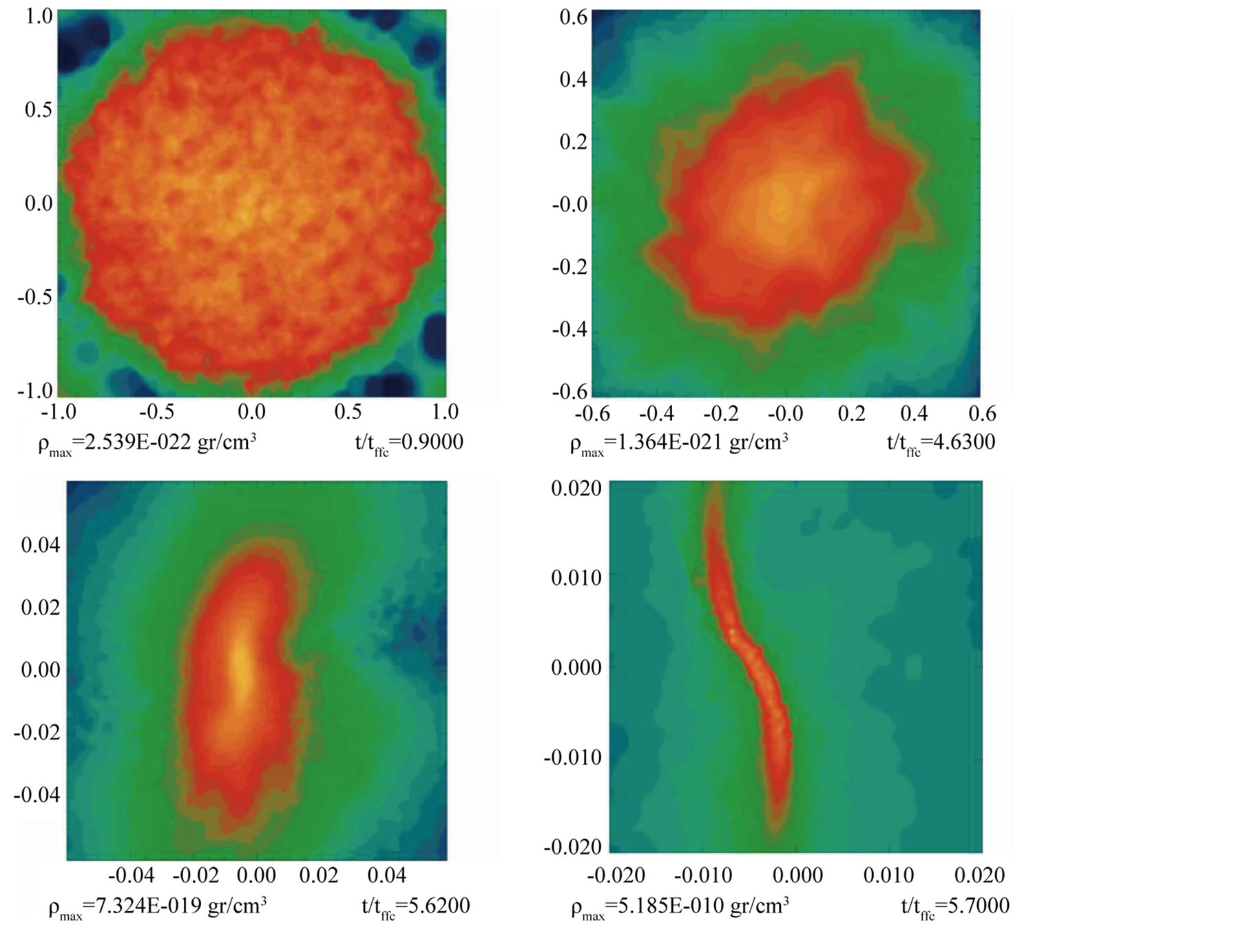
Figure 3. Isodensity plot illustrating the gravitational collapse process of the isolated and rotating cloud which we shall collide. We recall that  sec = 1.846 Myr.
netic energy into heat, as was described in the last paragraph of Section 2, that is radiated away in a very short timescale and we can assume that the shock and the clouds remain isothermal. During this process the kinetic energy and heat lost by the system makes it possible to approach equilibrium thereby increasing the fragmentation probability.
During the collision process a slab of material is formed along the shock front. The clouds then expand but eventually collapse as will be later described. The shocked slab which is formed as a result of the supersonic collision is susceptible of having various instabilities, which has been studied by [37] for the linear regime and by [38] for the non-linear case.
For the present work the relevant ones are the shearing and gravitational instabilities. The shearing instability dominates at low density while the gravitational one takes over for densities above the critical density
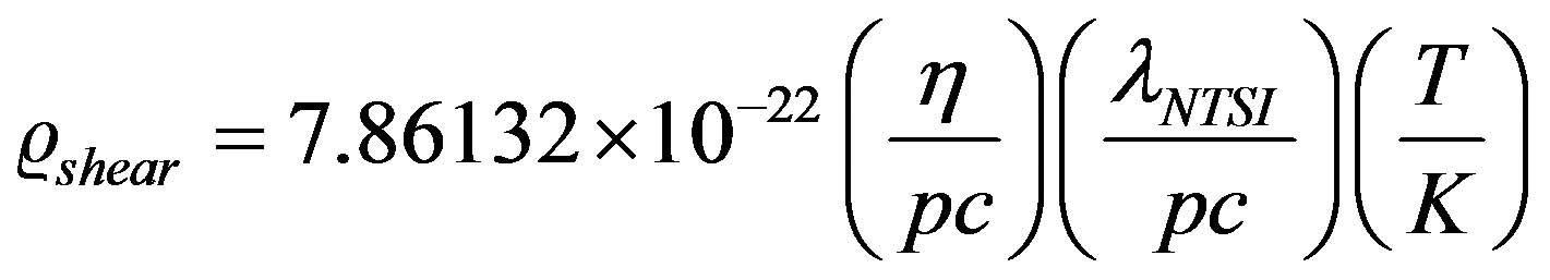 gr∙cm−3(13)
where  is the amplitude of the perturbation,
  the length of the unstable mode and T the temperature [39] .
Among the shearing instabilities the main ones are the non-linear thin shell instabilities (NTSI) and the Kelvin-Helmholtz (KH) instability.
The NTSI instability is expected to occur in the shocked slab just after the cloud collision, where non-linearbending and breathing modes could also be present.
4.3. The Head-On Collisions
In order to study the collision process when the approaching speed increases, we have considered five head-on collision models: in the five models H0-1, H0-2, H0-3 andH0-5, the rotating clouds are approaching each other; while for model HONR-4 the colliding clouds have not been endowed with initial rotation.
The same approaching velocities were chosen for models H0-3 and HONR-4 in order to study the effect of cloud rotation on the collisions.
In the head-on collision models, two identical clouds are placed in contact barely touching each other. Each cloud shares some of its particles which are closer to the edge of the neighboring cloud. Due to gravity and the approaching velocity the clouds collide producing a compression first, that is followed by an expansion. During this phase a contact layer forms between the clouds that thickens as the approaching speed of the clouds increases. A shock wave propagates into the clouds producing a collection of filaments and clumps that can be seen in the top left panel of all the evolution plots. The expansion of the clouds is eventually stopped by gravity and the collapse phase begins.
Just after the collision, a filament or slab of colliding particles quickly forms emphasizing the interface of the clouds. This is the phase where the slab may experience the NTSI and KH instabilities. From our numerical results we estimate that the parameters in Equation (13) are  and T = 10 K, and so the NTSI and KH instability are suppressed when the density goes above
  gr∙cm−3.
In the next three head-on collision models the clouds approach each other with increasing velocities. In model H0-1, we have ; we show the evolution of this model in Figure 4. Model H0-2 has an approaching speed of
  and its evolution can be seen in Figure 5. For
  we have two cases, model HO-3 whose iso-density plot is shown in Figure 6, and the initially non-rotating model HONR-4, shown in Figure 7.
Finally, the highest approaching speed we have considered is , which corresponds to model HO-5 whose isodensity plot is presented in Figure 8.
We notice that as we increase the approaching velocity of the clouds, the bridge that forms in the interface
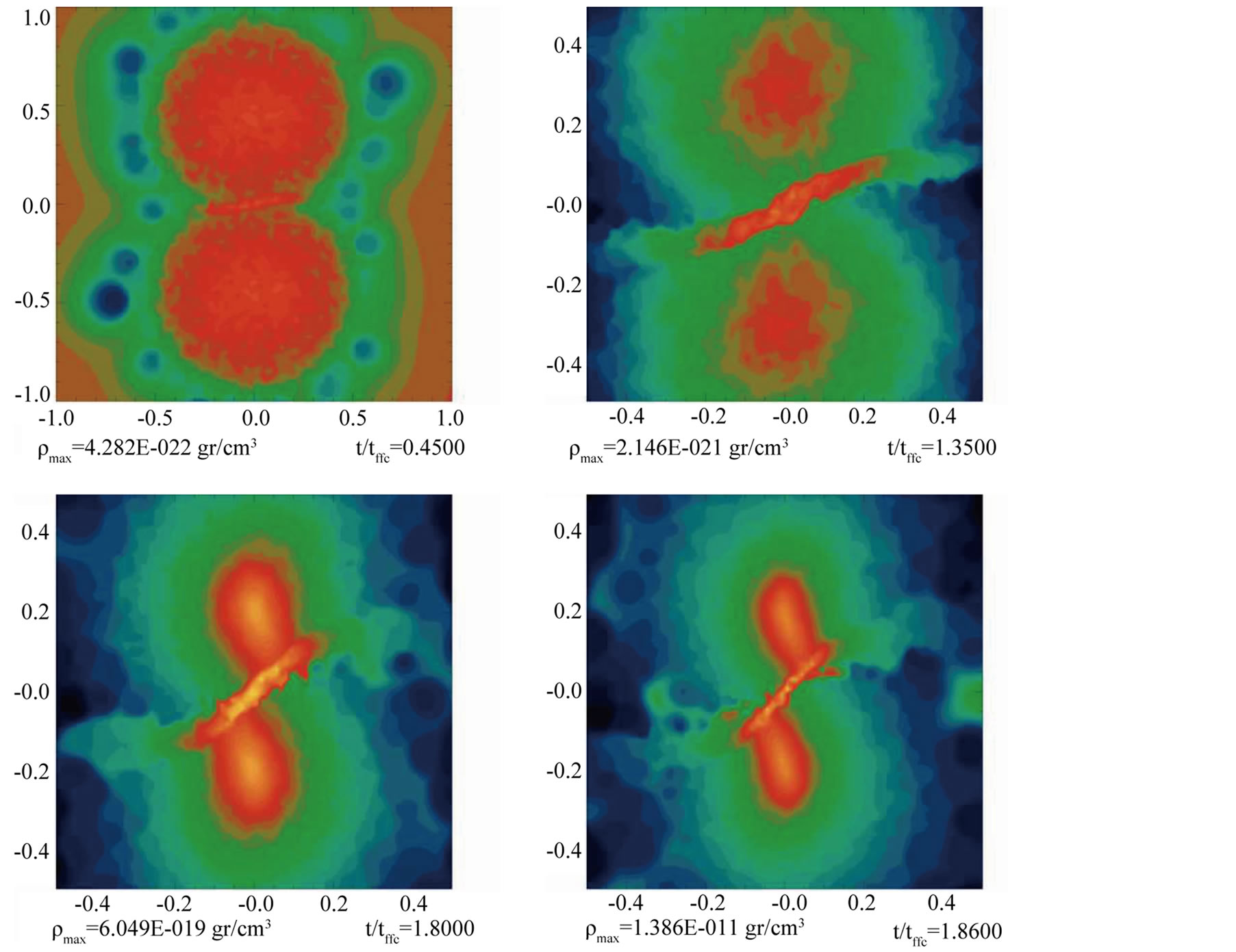
Figure 4. Isodensity plot for model H0-1.

Figure 5. Isodensity plot for model H0-2.

Figure 6. Isodensity plot for model H0-3.
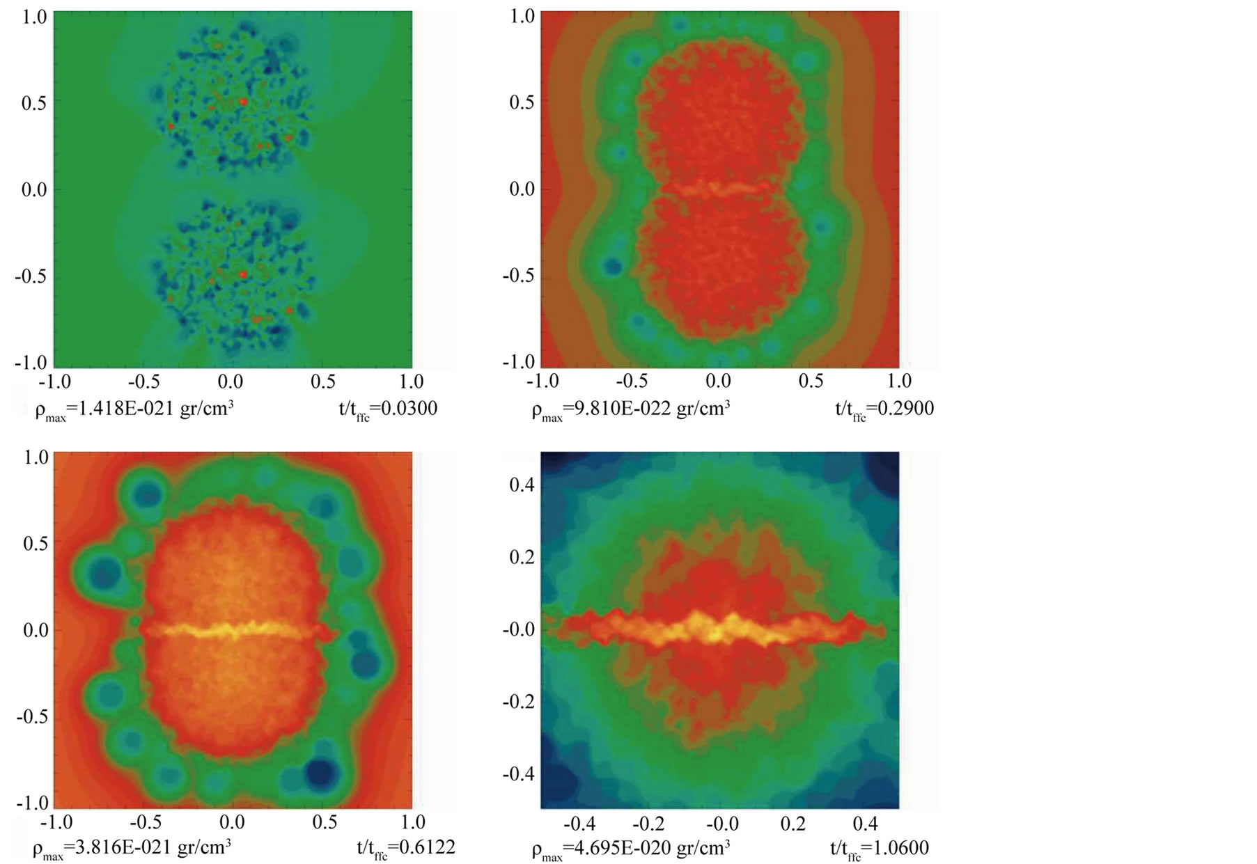
Figure 7. Isodensity plot for model H0NR-4.
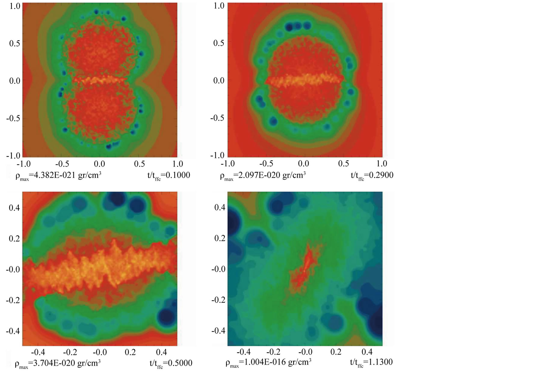
Figure 8. Isodensity plot for model H0-5.
becomes larger and thicker while the effect of the cloud’s self-gravity is less important. This indicates that many particles from the clouds are flowing very quickly to the bridge, to the point that the two initial clouds cannot be distinguished anymore in model HO-3 after a time of . For model HO-3 the final effect of the collision is to replace the two initial colliding clouds by a single cloud that more rapidly collapses towards a long filament.
It is interesting to notice the bending of the bridge in all these models; this bending is due to the individual rotation of the clouds. In model H0NR-4 all the matter collides in the interface of the clouds forming a longitudinal filament as is shown in Figure 7. For the purpose of comparing the result of our 3D simulations with Fig. 38 of [8] , in Figure 9, we zoom the filament that results from model H0NR-4. The density contours and the velocityfield in this figure suggest the appearance of bending and KH instabilities.
During the initial phase after the collision, the cloud’s peak density wiggles in time, as can be observed for model H0NR-4 in the top panels of Figure 10. These wiggles are a consequence of the density shock developed after the clouds collision in the mid plane. For model H0-3 we have also found the presence of density wiggles although of a smaller amplitude, see the bottom panels of Figure 10.
To understand the effect of an even higher approaching velocity, we have included model H0-5 with an approaching speed of 30.78 times the sound speed. As expected the density shock is stronger and in Figure 8 we sketch its evolution. Again we observe the formation of a strong filament in the interface of the clouds that rapidly expands as a strong flow of particles reaches the filament ends. However, the expansion eventually stops and the filament bounces back to begin the expansion in the transversal direction, along the Y-axis. This behavior has been previously observed by [4] .
The density wiggles are shown in the fourth panel of Figure 10. For the sake of looking for other kinds of instabilities in model H0-5, we have also included some plots with velocity distributions in Figure 11.
For the collision systems considered the initial and final values of α, β and α + β are shown in Table 1. For the initial head-on configurations, α + β increases from 0.404 for model HO-1 to 15.247 for model HO-5, which is a very high number and a consequence of the high Vapp value of Mach 30.78. In all head-on models a large fraction of the translational kinetic energy is transformed into heat and is radiated away. This is the reason why the Final α + β values reach the equilibrium value of 0.5.
4.3. Oblique Collisions
The oblique collisions are characterized by an impact parameter b which depends on the initial radius R0 of the cloud. The model with the smallest b has , while that with the largest b has b = 2.0R0.
The sign of b is important because it determines the initial orientation of the colliding clouds as we now explain.
For instance, for model M1 with the smallest b, we have placed the first cloud such that its center of mass in rectangular coordinates is , while the center of mass of the second cloud is
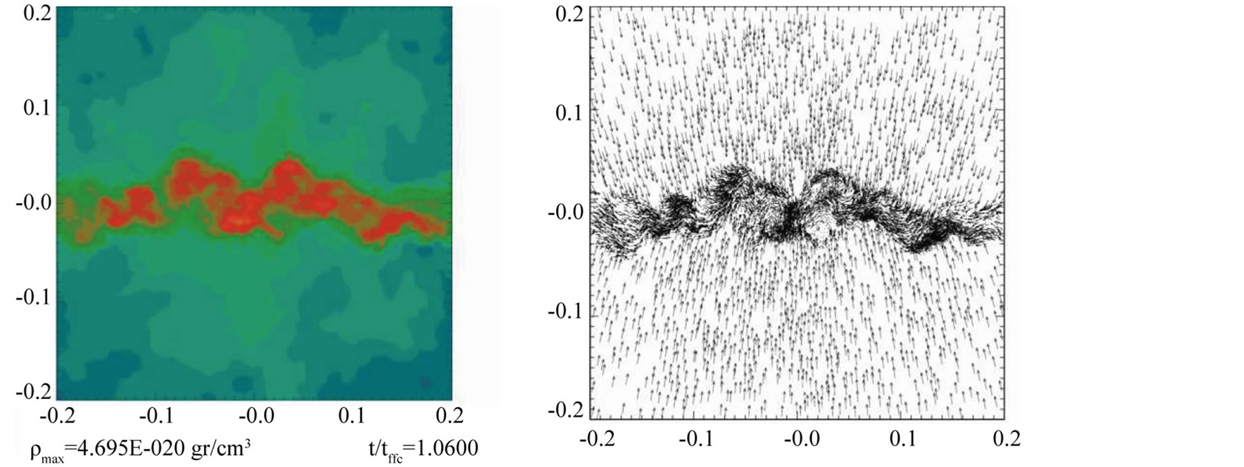
Figure 9. Zoom in of the filament of model H0NR-4 as it is shown in the last panel of Figure 7. We show isodensity curves (top panel) and the velocity field (bottom panel).

Figure 10. Time evolution of the peak density in the midplane of the collision for the XZ plane (continuous line), and for the entire collision volume (dashed line), for model H0NR-4 (top-left panel and zoomed in top-right panel), model H0-3 (bottom left panel), and model $H0-5$ (bottom right panel).
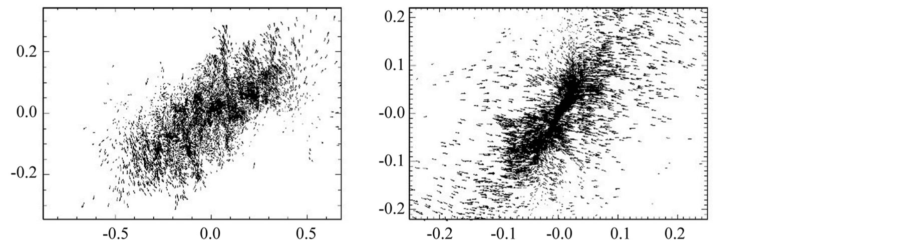
Figure 11. Velocity distribution in the XY plane for model H0-5 for  and
and  gr cm-3 (top panel), and
  gr∙cm−3, which corresponds to the last frame of the isodensity plot shown in Figure 8 (bottom panel).
 . We consider this orientation to correspond to a positive impact parameter b as labeled in the second column of Table 1. In this configuration the clouds are moved along the X-axis in the same sense than their rotational motion. For the opposite case, when b < 0, the clouds are again displaced along the X-axis, but in the opposite direction to its rotation.
As expected, the result of the collision for model M1 is quite similar to that obtained for the head-on low approaching velocity collisions. Indeed, the outcome of this model is very similar to that obtained for model HO-1, because the approaching speed of these two models is almost equal, see Figure 12. It is unnecessary to calculate more models with increasing Vapp with this impact parameter because we would expect that the results are very similar to those obtained for the head-on collision models.
Let us now consider models M2 and M21, where the impact parameter has been increased to b = R0, again with the positive orientation. The approaching velocity for the later is almost three times that of the former, with velocities given numerically by  and
and , respectively. As expected, in these two models the size of the bridge of particles inthe colliding interface is very sensitive to the approaching speed value. Whereas in model M2, it is always possible to distinguish the form of the two colliding clouds, in model M21, it is clearly seen that the participating clouds tend to merge, while the bridge becomes larger and thicker, see Figure 13 and Figure 14, respectively.
In model M21, the lack of time for self-gravity to act on the clouds is evident. On the other hand, the results for models M2, HO-1 and M1 are very similar because self-gravity had enough time to act on all of them prior to the collision. It is instructive to compare the outcome of models HO-3 and M21, whose approaching velocities are very similar. In both models the bridges have a similar size, although their orientations are quite different as a consequence of the impact parameter of model M21, see again Figure 6 and Figure 14 for a comparison.
For models M3 and M31 we have not increased the magnitude of the impact parameter, but we have changed its sign as well approaching speeds. The rectangular coordinates of the center of mass for the colliding clouds are now  and
and , respectively. That is, we now have b = −R0, see Table 1. The magnitude of the approaching speed for these models is
  and
and , respectively. This orientation will also be used for the next models. One of the most interesting evolutions is produced by model M3, as can be seen in Figure 15. In this case, the bridge starts forming in an inclined orientation and it ends up almost vertical along the colliding symmetry axis (the Y-axis); besides, it is much thicker and smaller
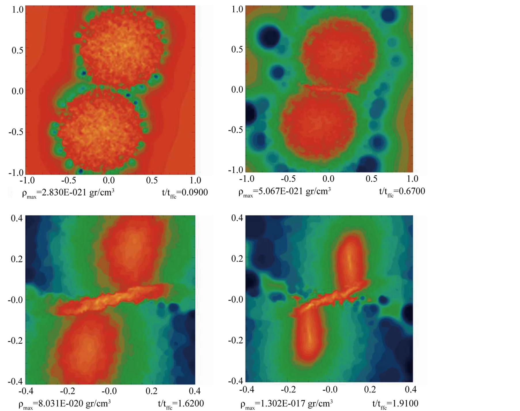
Figure 12. Isodensity plot for model M1.
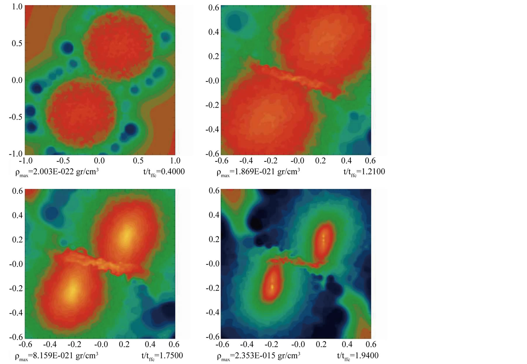
Figure 13. Isodensity plot for model M2.
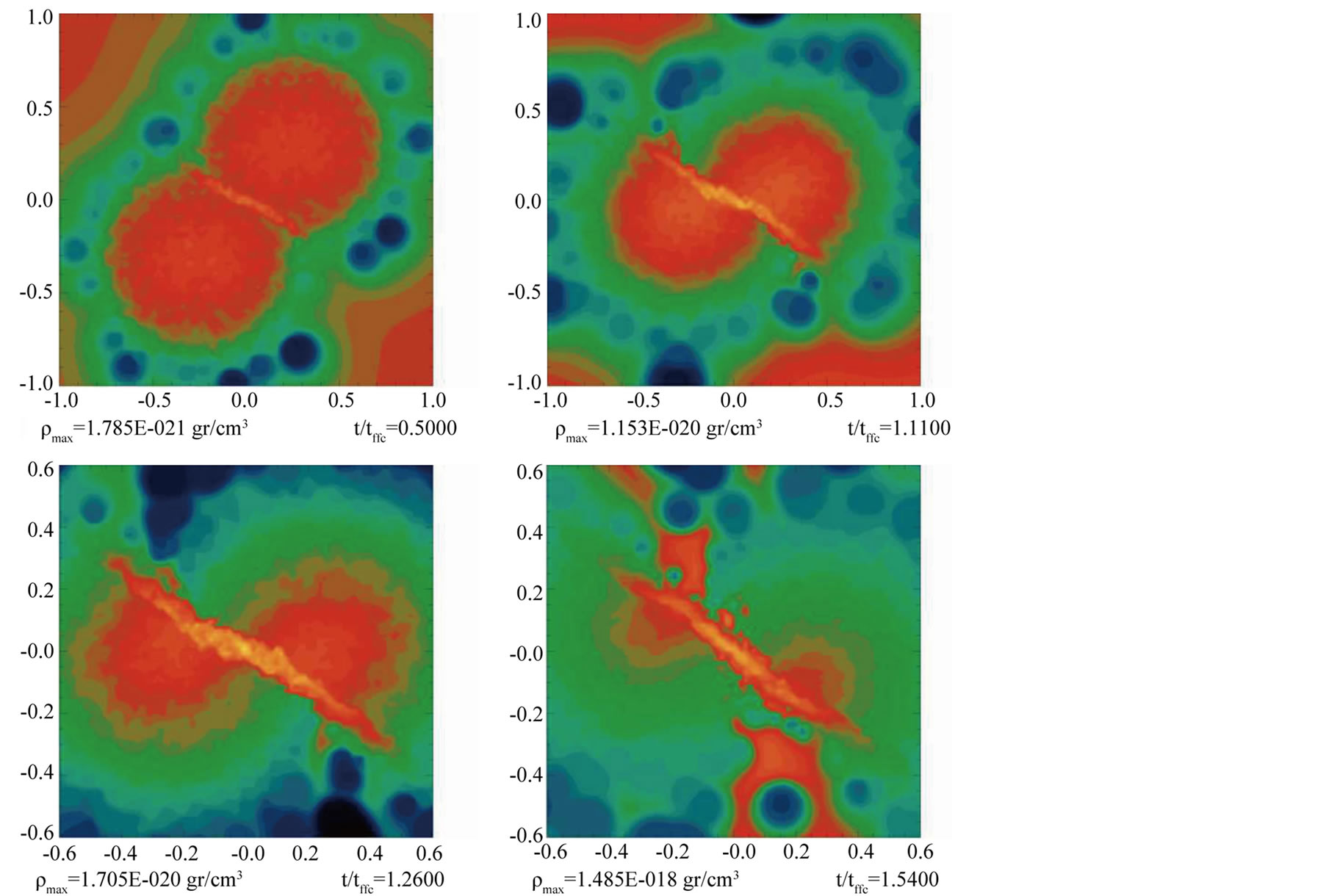
Figure 14. Isodensity plot for model M21.

Figure 15. Isodensity plot for model M3.
than in all the previous cases. We will describe in Section 4.5 the final evolution. As usual, the next model M31, has the same initial orientation than model M3, but we have almost doubled its approaching speed. The outcome of model M31 is quite different to that of model M3, as can be seen in Figure 16. For the last models labeled M4 and M41, we further increase the impact parameter b up to the value of −2.0R0.
We observe that depending on the magnitude of the approaching speed, the bridge of particles in the interface of the colliding clouds can remain and act as a gravitational link between the clouds, as can be seen in Figure 17 and Figure 18; or when this approaching velocity is sufficiently high, the clouds move next to each other and the bridge disappears, see Figure 19.
It turns out to be very interesting to analyze the initial and final α, β and α + β values for the oblique models, see This is not the case for the oblique models, which have a final near equilibrium value for Vapp less than about Mach three and all b values.
The final α + β values do not reach the equilibrium for Vapp greater than eight and high b values. Hence we only get very high dissipation for head-on or near head-on collision.
4.4. Physical Properties
In this section we describe the integral properties of the clumps or fragments found in some of our simulations; properties which characterize the physical state of the resulting clumps, among others, the energy ratios α and β already defined in Equation (5).
We first proceed to find the center of the clump which is given by the location of the particle with the highest density in the region where the clump is located. With the clump center determined, xcenter, we then find all the particles which have a density above (or equal to) some minimum density value ρmin and that, at the same time, are located within a given maximum radius rmax from the clump center. With this set of Ns particles we can estimate the integral properties of the clump.
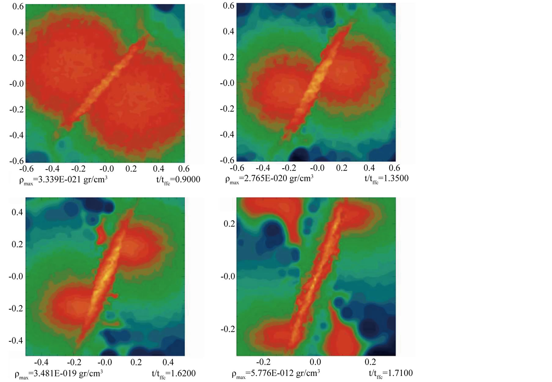
Figure 16. Isodensity plot for model M31.
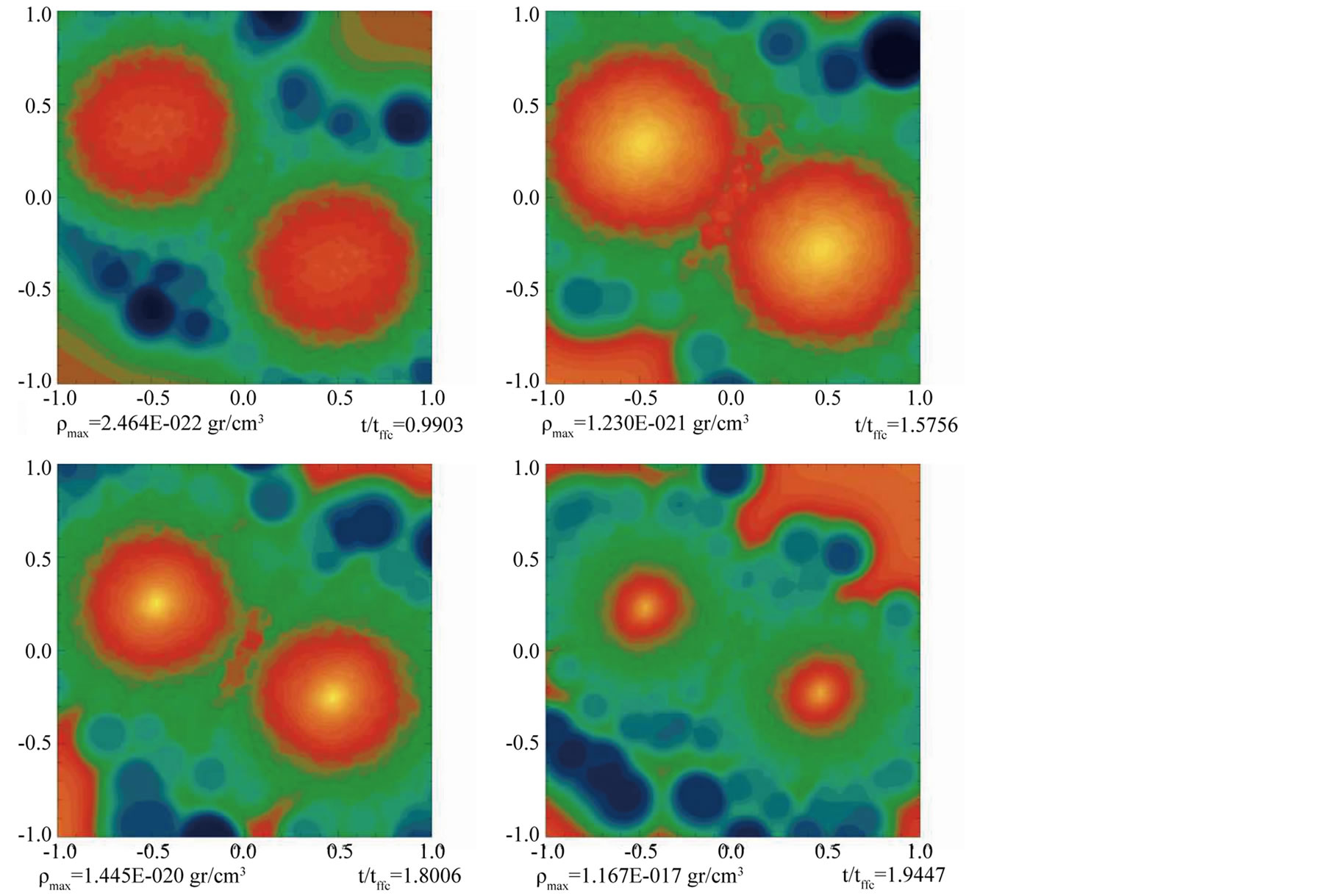
Figure 17. Isodensity plot for model M4.

Figure 18. Isodensity plot for model M41.
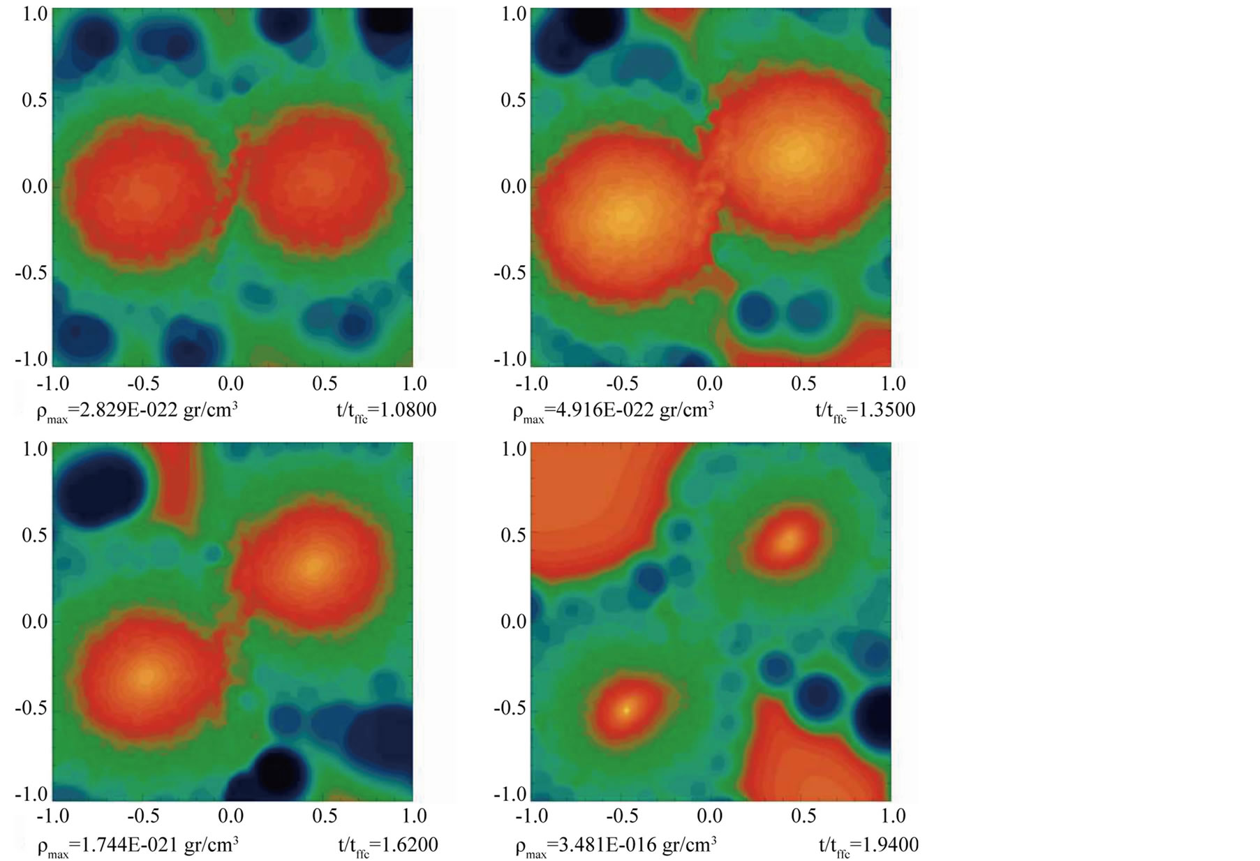
Figure 19. Isodensity plot for model M42.
We use the smoothing kernel for calculating the density of particle i by means of , where
  is the spline kernel given in Equation (A1) of [40] . For the gravitational potential, we use another kernel such that
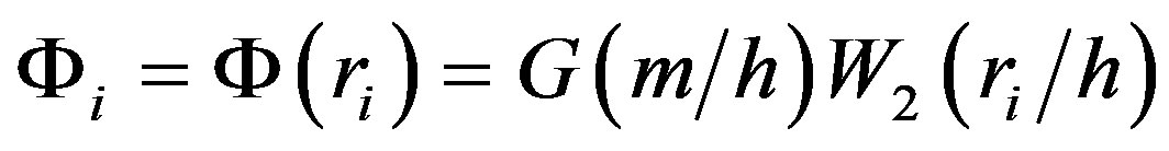 , where the kernel W2 is now given in Equation (A3) of the same reference. The softening length h appearing in these two kernels, sets the neighborhood on the point r outside of which no particle can exert influence on r, that is, for r > h both kernels vanish: W1 = 0 and W2 = 0. We use several values for h, with the purpose that the number of neighbor particles for any point (or particle) be near 50.
The next step is to make a sum over all the set of Ns particles, from which we obtain the density and the gravitational potential for every particle  due to the presence of all other particles j ≠ i. We keep Ns to be around 100,000 particles. Then we approximate the thermal energy of the clump, by calculating the sum over all the Ns particles, that is
 (14)
(14)
where P is the pressure associated with particle i with densityρi by means of the equation of state given in Equation (7). In a similar way, the approximate potential energy is
 (15)
(15)
Although a bit more complicated, the rotational energy of the set of Ns particles is calculated with respect to the Z-axis of the located clump, as follows. Let xi and vi be the position and velocity of particle i. Then the coordinates of those particles in the clump with respect to the clump center are . The azimuthal angle
  associated with the rotation of particles with respect to the Z-axis can be calculated by taking the ratio of the projection of coordinates of the particle with the unitary vectors i = (1,0,0) and j = (0,1,0), that is we can write
 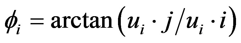 . Therefore the angle
  also depends on the particle i, that is,
 . Then the rotational energy can be estimated by taking the projection of the velocity along the unitary azimuthal vector
 , that is
 (16)
(16)
We report in Table 3 the results obtained by the application of the preceding calculation procedure to the lastsnapshot obtained in each simulation. It must be noted that the numerical results for integral properties unfortunately depend on the values chosen for two cutting parameters, ρmin and rmax, therefore we inevitably commit certain ambiguity in defining the clump boundaries. For instance, the minimum density is fixed arbitrarily. We will next describe the entries of Table 3 as follows (see the next page).
In column one, we repeat the label of the model as many times as needed to account for all the identified clumps in the model. In column two we indicate the number of particles (Ns) entering into the set of particles that approximate the physical state of the clump with respect to the energy calculation. In columns three, four and five we show the Cartesian coordinates of the center of every identified clump, expressed in terms of the side length of the simulation box, 2R0. Later on, in column six we show the ratio of the minimum density to the initial central density of the cloud, which is the lowest value that a particle entering in the set can indeed have. In column seven we indicate the maximum radius in units of 2R0. In column eight we show the softening length h in units of R0. In columns nine and ten we present the energy ratios α and β as previously defined, and finally in the last column we add α + β. In Table 4 we show for some models the peak velocity in sound speed units (Mach number) and the maximum acceleration normalized with as = 3.64 × 109 cm∙s−2. For almost all models the maximum velocity is about Mach 10 and since quite large maximum accelerations are reached, this makes the computational time step to get very small. Because of this in some models the evolution cannot be followed to very high density.
For model HO-1 the first and second fragments have α = 0.19, 0.23, β = 0.12, 0.13, and α + β = 0.315, 0.366, respectively. The fragments have already collapsed by ten orders of magnitude in density, and the low α + β values suggest that they will continue to do so, inhibiting any further fragmentation. The β values are very low because the collision is head-on. The original clouds have β = 0.16134 and as a result of the collision is reduced to about 0.12 - 0.13. The central filament rotates as a consequence of the initial rotation of the clouds, it contains
Table 3. Physical properties of the resulting protostellar clumps.
Table 4. Peak values for the velocity (normalized with the sound speed) and the acceleration (normalized with as = 3.64 × 109 cm∙s−2 obtained for the last snapshot of some representative runs.
the highest density regions and fragments into several clumps. For the oblique collision model M1, the impact parameter b/R0 = 1/2 and the approaching velocity is Vapp = 2.52 co, see Figure 12. The fragments in the last panel of this figure are well defined, one is binary (top-right) and the other one single (lower-left). The fragments have shifted from the original head-on collision alignment because of the impact parameter b, but also as a result of the rotation of the clouds which is counterclockwise. The α + β values of the two fragments are 0.86 and 0.90, respectively. These numbers are well above the virial value and the system at the last computed time step has only been able to increase its density by about five orders of magnitude. Both fragments need to lose a significant amount of angular momentum for the collapse to proceed at a faster rate. The central filament is well defined, its maximum density is similar to that of the fragments and at the last computed model shows signs of fragmentation. From Figure 20 we observe that there is a flow of particles going in all directions, as can also be seen in Figure 21 where we sketch the 3D bridge structure.
Model M2has some similarities to model H0-1, compare the last frames of Figure 4 and Figure 13. The fragments for model M2 are more detached from the filament, which is due to the combination of the initial angular velocity of the clouds and its initial condition that corresponds to an oblique collision with an impact parameter b/R0 = 1/2. For the HO-1 case the fragments are less detached from the filament because we only have the contribution from the initial angular velocity of the clouds. The central filament is dissolved, and it can only survive if the impact parameter b/R0 is low (<1/2).
Model M2 is very interesting because as we shall see, it produced two filament-like fragments that appear to be subfragmenting. In Section 3.4 we showed that the Jeans length criterion is satisfied for all models. Despite
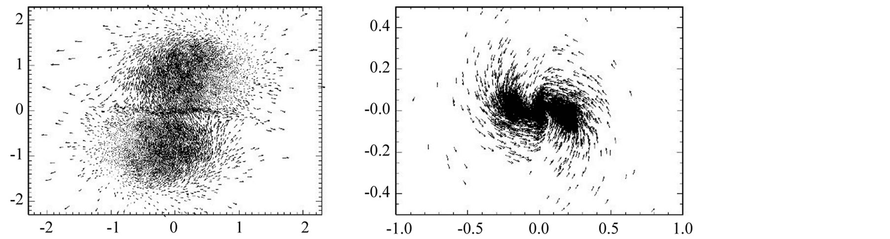
Figure 20. Velocity field for the last snapshot obtained for models M1 (top panel) and M3 (bottom panel).
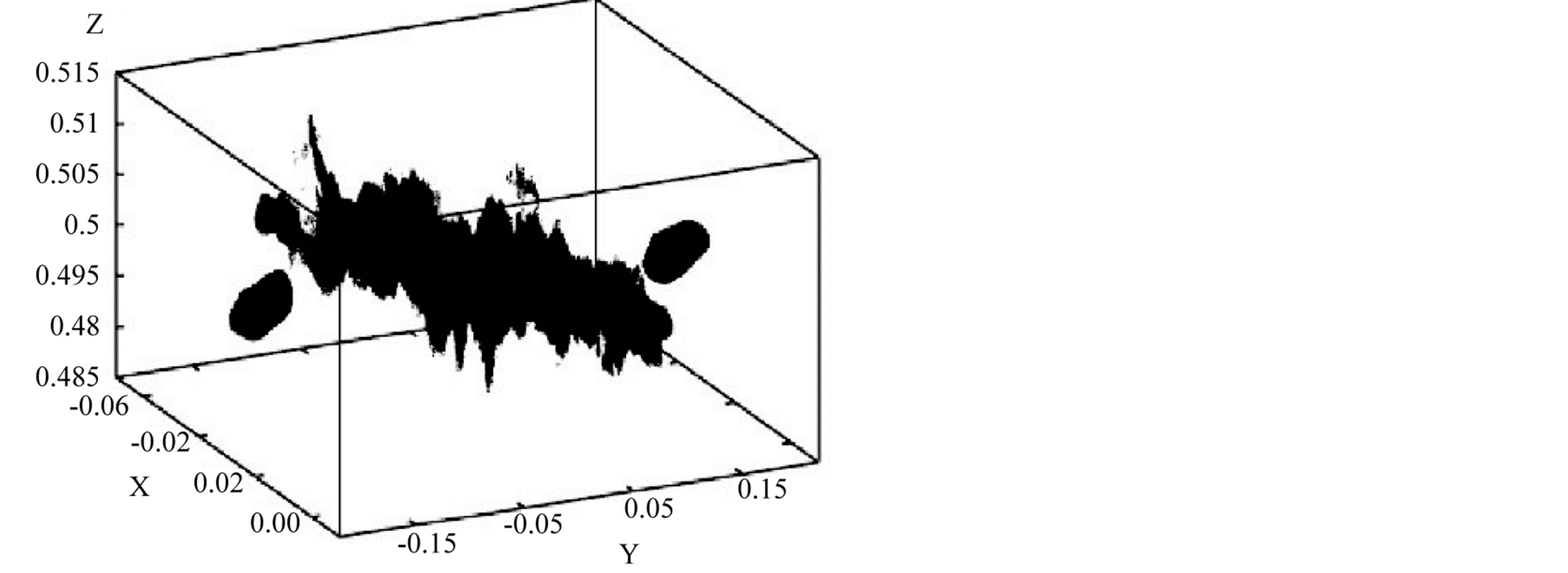
Figure 21. Dot plot for the last snapshot obtained for model H0-1 when t = 1.863655τff and log10(ρmax/ρ0) = 10.93. In this plot each dot represents an SPH particle and only thoseparticles having log10(ρ/ρ0) > 2.5 have entered, which are 800,566, that is, only 8 percent of the total number of particles.
this, in order to ensure that the result of model M2 is not affected by artificial fragmentation, we simulated again this model with 15 million particles, this represents 50% more than for the rest of the models and basically obtained the same result. In Figure 22 we show an amplification of the resulting system of the resimulated model M2 for the last computed time step. We refer to the two fragments as top-right and lower-left. The filament-like structure of the two fragments is produced by the initial compression of the clouds that generates a density maximum along a line parallel to the collision shock front and at the center of the clouds.
This is an initial condition very different from the standard m = 2 perturbation, see Equation (6). If clouds do not experience a strong direct collision, that is, if the impact parameter b/R0 > 2, or the separation of the clouds is much greater than their radius, the induced perturbation is a mixture of an m = 2 and m = 3 perturbation, but if the collision is strong and b < 1 the perturbation is filament-like.
An amplification of the top-right and lower-left fragments of Figure 22 shows that they have sub fragmented into several clumps. For the lower-left fragment α = 0.110, β = 0.392, and α + β = 0.501, that is, the system composed by this fragment has virialized, the collapse has stopped completely and the newly formed fragments are expected to become stars after they reach higher densities. For the top-right fragment α = 0.108, β = 0.433, α + β = 0.541, and the system is also close to virial equilibrium.
Model M3 for which b/R0 = −1 and Vapp = 4.58c0 evolved into two single fragments and the filament decayed into a central fragment see Figure 15. For the central fragment, from Table 4, α + β = 0.36, and so we expected that it will continue collapsing to much higher densities. The outer two fragments have α + β = 2.016 and 1.752, respectively, and in particular, very high rotation energies, so for them to be able to collapse it is required that they lose large amounts of angular momentum. The velocity field for this model is shown in Figure 20, from where we can appreciate that many particles are orbiting around the system in circular orbits but not really col-
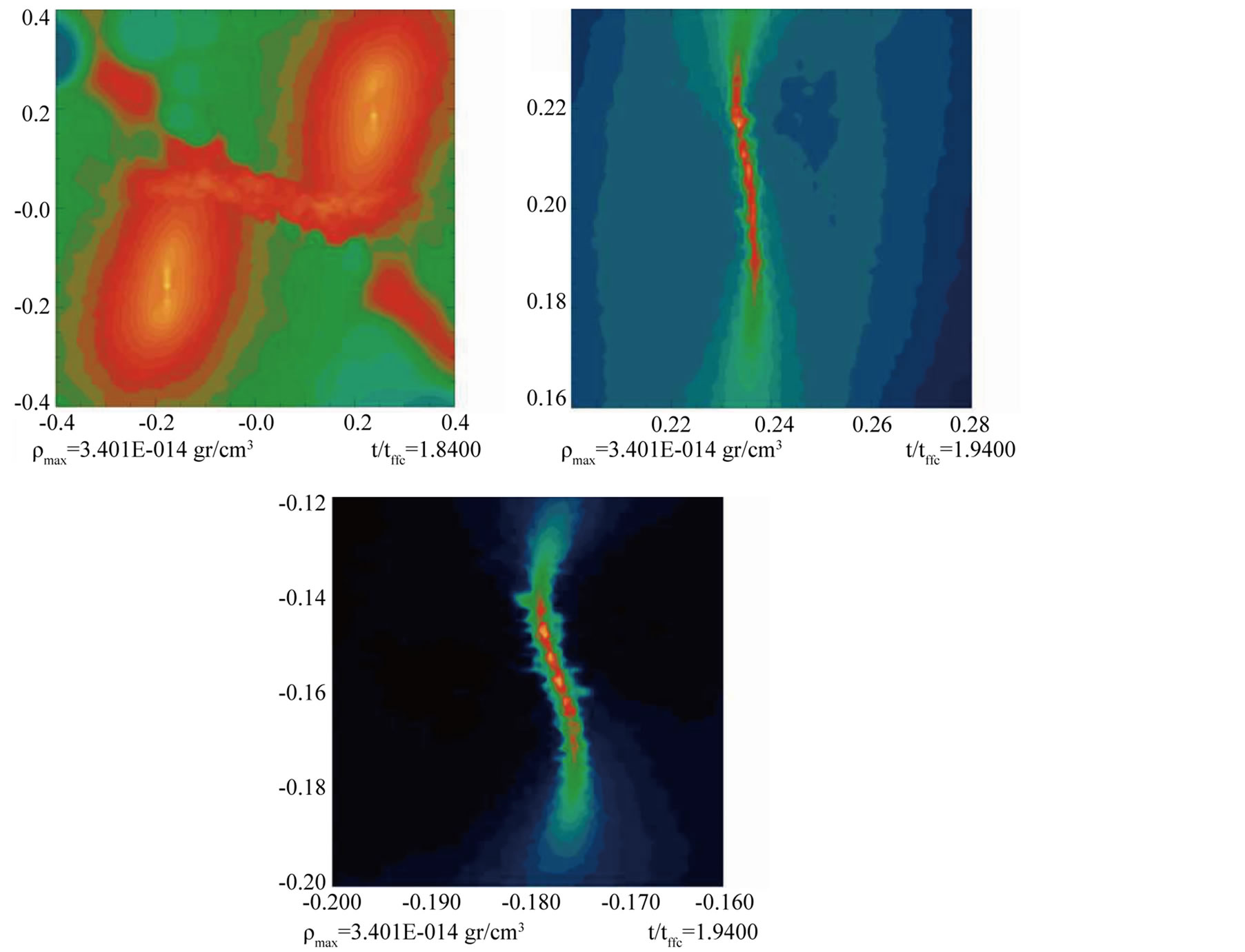
Figure 22. We show here an amplification of the last snapshot obtained for a resimulation of model M2 which should be compared with the last panel of Figure 13 (top panel), and of this panel a further amplification of the top-right filament (middle panel), and of the lower-left filament (bottom panel).
lapsing. The small b and quite high Vapp produce the very high rotational velocities in the outer fragments.
We now describe model M4 that has b/R0 = −2.0 and Vapp = 2.74c0. The two outer fragments are single, well defined, and have α + β = 0.4986 and 0.53105, respectively, which is very close to the virial value of 0.5. The fragments require to lose thermal and rotational energy to be able to reaching higher densities. The central filament quickly disappears because of the high b value. Model M41 with b/R0 = −2.0 and Vapp = 4.58c0 has a similar revolution to model M4 which has the same b but lower Vapp. The α value of the fragments is about 0.21 but the β value is above 0.60 which makes α + β take values above 0.82 and so the fragments need to get rid of some angular momentum to be able to collapse. The higher angular moment is generated during the collision as a result of the higher Vapp.
The velocity and acceleration particle distributions for some of the models are shown in Figure 23. In this figure f means the fraction of particles in the simulation which have a velocity (left panel) and an acceleration (right panel) less than the number indicated in the horizontal-axis, respectively. We show in Table 4 the maximum values for velocities and accelerations obtained for the last snapshot of some simulations.
5. Discussion
In this paper we carried out a fully 3D set of numerical hydrodynamical simulations within the framework of the SPH technique, aimed to follow the collision process of two small rotating uniform density clouds.
The initial conditions for the isolated cloud are such that it will collapse in the absence of a collision. However, when we consider the translational kinetic energy that comes from the approaching velocity Vapp of the clouds, the collision system is unbound for Vapp greater than about three, that is, (α + β)initial > 0.5, see Table 1.
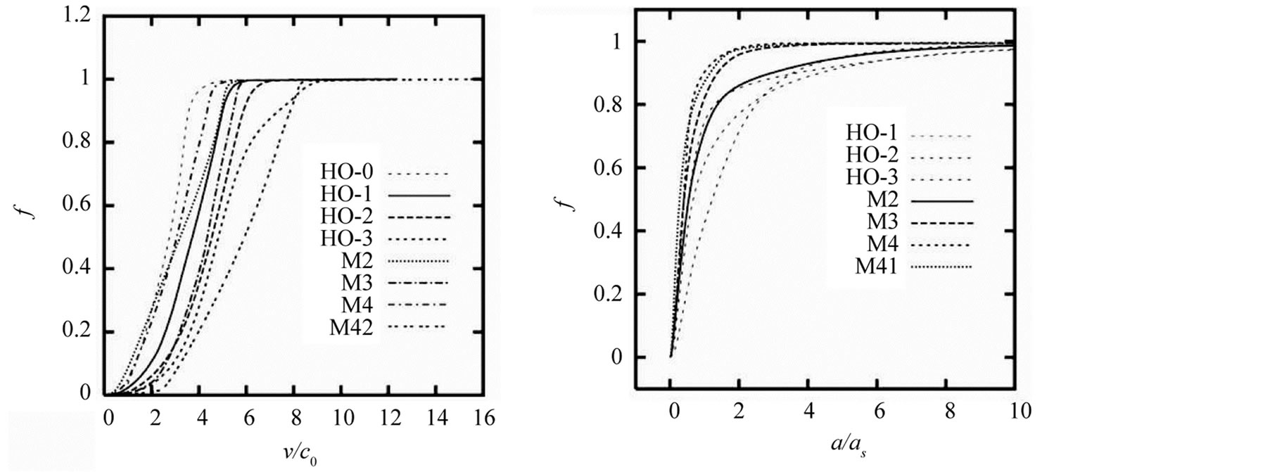
Figure 23. Fraction of particles f having less than or equal to the peak velocities as indicated in the X-axis (top panel); the peak accelerations expressed in terms of as = 3.64 × 10⁻⁹ cm/sec2 (right panel).
As a result of the collision process a large fraction of the translational kinetic energy is transformed into heat that is radiated away because the clouds and the shock front that forms in the inter phase between the clouds are isothermal. This produces a reduction of the global value of α + β for all models. For the head-on models we found that they all get a final configuration near equilibrium even for very high Vapp. This is not the case for the oblique models, which have a final value near equilibrium for Vapp less than about Mach three and all b values. The final α + β values get away from equilibrium for Vapp greater than eight and high b values. Hence we only get very high dissipation, and thus the possibility of fragmentation for initially unbound systems for head-on or near head-on collision.
When the cloud collides, the gravitational collapse speeds upin some regions and we do observe fragmentation in some of the models, see for example Figure 13 and Figure 22. This result is different from that of [13] that found that most supersonic head-on cloud collisions will probably do not result in fragmentation, unless the interstellar gas can cool much faster than it is normally assumed. They concluded that most cloud collisions produce a disruption or dispersion of the clouds involved.
In this work we have observed that the result of simulation depends mainly on two physical factors that compete to exert more influence on the collision process. These factors are self-gravity and the flowing of particles from the colliding interface. The occurrence and extension of these effects are regulated by the value of the approaching velocity of the colliding clouds.
The two cloud collision forms a shock front, the clouds are first compressed but then expand. In all simulations the shock front produces a collection of filaments and clumps, and the bending and KH instabilities are observed for densities lower than about 10−18 gr∙cm−3, i.e. before the collapse is truly underway.
With no collision or with a very slow approaching velocity, self-gravity dominates the evolution of both clouds. In these cases, the main effect of self-gravity on the system is the decreasing size of each of the clouds. The collision system quickly reaches a configuration in an advanced state of gravitational collapse consisting of two gas clumps (the cores of the clouds) linked by a bridge of matter. In some cases the clumps or fragments have sub-fragmented into an elongated filamentary structure that is very close to virial equilibrium. Besides that, there is always a sharing region of particles between the clouds that gives place to the formation of a bridge of gas, even when no collision occurs.
On the other hand, when a collision takes place with a significant approaching velocity, self-gravity plays a minor role and the fate of the system is entirely determined by the strong flow of particles in the interface of the clouds. In these cases, the main effect on the system is to replace the two initial collapsing clouds by a single cloud that is rapidly shocked to give place to an elongated and irregular filamentary structure formed in the shock region. This filamentary structure increases its size very rapidly as it is continuously fed by in falling material coming from the original clouds.
The second important parameter of the collision process is the impact parameter b. For instance, it should be noted that for models with the same approaching velocity and with the same magnitude of the impact parameter b, but with a different sign of b, we have obtained different outcomes. We have tried to consider several parameters in order to make a representative study, but as the space parameter is very large, it cannot be covered in a single work.
It is interesting to note that the particle with the highest density in the simulations was not always found in the bridge of matter, but there were cases where it was located in the remnants of the clouds; remnants that hopefully will end up as protostellar cores.
For model H0-1, in Figure 21, we show in a dot plot the 3D structure of the bridge. Each dot represent an SPH particle and we have only included those that have a density greater than a certain value, which is given in the bottom of the figure. It can be appreciated that the bridge is highly irregular as many particles flow very fast in all directions, and are continuously ejected from the collision region.
In view of our simulations, the future of the bridge is as yet unclear; but it is likely that most of the gas is destined to remain in this filamentary structure as the collapse progress further. Although many clumps of matter get formed near the principal bridge, these clumps are very thin and small, then it could be the case that the diameter of these clumps are in general greater than the Jeans length. This is another reason why the bridge would not be an appropriate site for protostellar formation until it cools further.
As described in Section 3.4, the Jeans mass requirement is a necessary condition for avoiding the occurrence of artificial fragmentation. As far as we know, the only way to ensure the correctness of a simulation is by making a convergence analysis in which the total number of particles increases systematically.
Although this analysis is beyond the present manuscript, we have been careful to resimulate at least model M2 with 15 million particles, that is, 50% more than for the rest of the models.
In fact, in Figure 22 we show an amplification of the last snapshot computed in this resimulation of model M2. We have pleasantly found convergence.
The filament-like structure of the two fragments is produced by the initial compression of the clouds that generates a density maximum along a line parallel to the collision shock front and at the center of the clouds. This is an initial condition very different from the standard m = 2 perturbation, see Equation (6). If clouds do not experience a strong direct collision, that is, if the impact parameter b/R0 > 2, or the separation of the clouds is much greater than their radius, the induced perturbation is a mixture of an m = 2 and 3 perturbation, but if the collision is strong and b/R0 < 1 the perturbation is filament-like.
Besides, we note that the filament developed in the central region of each clump, show a clear tendency to fragment by forming small knots along the filament. This behavior contrasts with the fate of the filament developed for the initial cloud when it evolved as an isolated system, which shows no tendency to fragment, as can be appreciated in the last panel of Figure 3. We conclude that the fragmentation of the filaments in model M2 is a consequence of the collision.
6. Concluding Remarks
It was [40] who predicted that the infall of gas colliding into the galactic disk could have a huge influence on the star formation process, and at the same time, to inherit a very peculiar physical structure to the interstellar gas. It is already well known that recent observations show some elongated structures in the Orion Molecular Cloud, which appear to be common in the observed interstellar medium.
In this manuscript we have been able to capture and show some of the essential features of the collision process. For instance we have obtained irregular systems of filaments and clumps of neutral gas, which could be somehow compared with those already observed. We also investigated what are the physical properties of the resulting proto stars in this collision scheme, which hopefully could be compared with observations. Moreover, we claim to have observed some kind of fragmentation in the filaments of model M2, which is a direct consequence of the occurrence of the collision. This result can be considered as an evidence that collisions may have an important influence on the star formation process.
Calculations have been performed by colliding two identical polytropes (with their surfaces just in contact including self-gravity and viscosity) with the purpose to test the conservation of energy in codes based on the SPH technique [41] . They found that the errors in the non-conservation of energy can reach as much as 10 per cent values when the derivative of the h terms is not included in the particle equation of motion. Since the public version of the Gadget2 code used here does not include these terms we are at the worse non-conserving energy scene. Consequently, large errors in the system energy evolution are then expected.
Acknowledgements
We would like to thanks ACARUS-UNISON, KanBalam-UNAM, the Instituto Nacional de InvestigacionesNucleares and Cinvestav-Abacus for the use of their computing facilities. This work has been partially supported by the Mexican Consejo Nacional de Ciencia y Tecnología (CONACYT), Project CB-2007-84133-F. J. K. thanks the Consejo Nacional de Ciencia y Tecnología of Mexico (CONACyT) for partial support under the project CONACyT-EDOMEX-2011-C01-165873.
References
- Scoville, N.Z., Sanders, D.B. and Clemens, D.P. (1986) High-Mass Star Formation Due to Cloud-Cloud Collisions. Astrophysical Journal, 310, L77-L81. http://dx.doi.org/10.1086/184785
- Wang, J.J., Chen, W.P., Miller, M., Qin, S.L. and Wu, Y.F. (2004) Massive Star Formation Triggered by Collision between Galactic and Accreted Intergalactic Clouds. Astrophysical Journal, 614, L105-L108. http://dx.doi.org/10.1086/425657
- Burkert, A. and Alves, J. (2009) The Inevitable Future of the Starless Core Barnard 68. Astrophysical Journal, 695, 1308-1314. http://dx.doi.org/10.1088/0004-637X/695/2/1308
- Anathpindika, S. (2009) Supersonic Cloud Collision. I. Astronomy and Astrophysics, 504, 437-460.
- Hausman, M.A. and Ostriker, J.P. (1978) Galactic Cannibalism. III—The Morphological Evolution of Galaxies and Clusters. Astrophysical Journal, 224, 320-336. http://dx.doi.org/10.1086/156380
- Lattanzio, J.C., Monaghan, J.J., Pongracic, H. and Schwarz, M.P. (1985) Interstellar Cloud Collisions. Monthly Notices of the Royal Astronomical Society, 215, 125-147.
- Kimura, T. and Tosa, M. (1996) Collision of Clumpy Molecular Clouds. Astronomy and Astrophysics, 308, 979-987.
- Klein, R.I. and Woods, D.T. (1998) Bending Mode Instabilities and Fragmentation in Interstellar Cloud Collisions: A Mechanism for Complex Structure. Astrophysical Journal, 497, 777-799. http://dx.doi.org/10.1086/305488
- Marinho, E.P. and Lepine, J.R.D. (2000) SPH Simulations of Clumps Formation by Dissipative Collision of Molecular Clouds. I. Non Magnetic Case. Astronomy and Astrophysics. Supplement Series, 142, 165-179.
- Smith, J. (1980) Cloud-Cloud Collisions in the Interstellar Medium. Astrophysical Journal, 238, 842-852. http://dx.doi.org/10.1086/158045
- Kitsionas, S. and Whitworth, A.P. (2007) High-Resolution Simulations of Clump-Clump Collisions Using SPH with Particle Splitting. Monthly Notices of the Royal Astronomical Society, 378, 507-524. http://dx.doi.org/10.1111/j.1365-2966.2007.11707.x
- Anathpindika, S. (2010) Collision between Dissimilar Clouds: Stability of the Bow-Shock and the Formation of Pre- Stellar Cores. Monthly Notices of the Royal Astronomical Society, 405, 1431-1443.
- Whithworth, A.P. and Pongracic, H. (1991) Cloud-Cloud Collisions and Fragments. In: Falgarone, E., Boulangeer, F. and Duvert, G., Eds., Fragmentation of Molecular Clouds and Star Formation, International Astronomical Union, Kluwer Academic Publishers, Berlin, 523-525. http://dx.doi.org/10.1007/978-94-011-3384-5_95
- Bergin, E. and Tafalla, M. (2007) Cold Dark Clouds: The Initial Conditions for Star Formation. Annual Review of Astronomy and Astrophysics, 45, 339-396. http://dx.doi.org/10.1146/annurev.astro.45.071206.100404
- Myers, P.C. and Benson, P.J. (1983) Dense Cores in Dark Clouds. II-NH3 Observations and Star Formation. Astrophysical Journal, 266, 309-320. http://dx.doi.org/10.1086/160780
- Plummer, H.C. (1911) On the Problem of Distribution in Globular Star Clusters. Monthly Notices of the Royal Astronomical Society, 71, 460-470.
- Whithworth, A.P. and Ward-Thompson, D. (2001) An Empirical Model for Protostellar Collapse. Astrophysical Journal, 547, 317-322. http://dx.doi.org/10.1086/318373
- Myers, P.C. (2005) Centrally Condensed Collapse of Starless Cores. Astrophysical Journal, 623, 280-290. http://dx.doi.org/10.1086/428386
- Arreaga, G. and Klapp, J. (2010) The Gravitational Collapse of Plummer Protostellar Clouds. Astronomy and Astrophysics, 509, A96-A111.
- Bodenheimer, P., Burkert, A., Klein, R.I. and Boss, A.P. (2000) Multiple Fragmentation of Protostars. In: Mannings, V.G., Boss, A.P. and Russell, S.S., Eds., Protostars and Planets IV, University of Arizona Press, Tucson, 675-701.
- Sigalotti, L.G. and Klapp, J. (2001) Gravitational Collapse and Fragmentation of Molecular Cloud Cores. International Journal of Modern Physics D, 10, 115-211. http://dx.doi.org/10.1142/S0218271801000706
- Boss, A.P., Fisher, R.T., Klein, R. and McKee, C.F. (2000) The Jeans Condition and Collapsing Molecular Cloud Cores: Filaments or Binaries? Astrophysical Journal, 528, 325-335. http://dx.doi.org/10.1086/308160
- Arreaga, G., Klapp, J., Sigalotti, L.G. and Gabbasov, R. (2007) Gravitational Collapse and Fragmentation of Molecular Cloud Cores with GADGET-2. Astrophysical Journal, 666, 290-308. http://dx.doi.org/10.1086/520492
- Arreaga, G., Saucedo, J., Duarte, R. and Carmona, J. (2008) Hydrodynamical Simulations of the Non-Ideal Gravitational Collapse of a Molecular Gas Cloud. Revista Mexicana de Astronomía y Astrofísica, 44, 259-284.
- Whitehouse, S.C. and Bate, M.R. (2006) The Thermodynamics of Collapsing Molecular Cloud Cores Using Smoothed Particle Hydrodynamics with Radiative Transfer. Monthly Notices of the Royal Astronomical Society, 367, 32-38. http://dx.doi.org/10.1111/j.1365-2966.2005.09950.x
- Spitzer, L. (1978) Physical Processes in the Interstellar Médium. Wiley, Hoboken.
- Bekki, K., Beasley, M., Forbes, D. and Couch, W.J. (2004) Formation of Star Clusters in the Large Magellanic Cloud and Small Magellanic Cloud. I. Preliminary Results on Cluster Formation from Colliding Gas Clouds. Astrophysical Journal, 602, 730-737. http://dx.doi.org/10.1086/381171
- Larson, R. (1981) Turbulence and Star Formation in Molecular Clouds. Monthly Notices of the Royal Astronomical Society, 194, 809-826.
- Chapman, S., Pongraic, H., Disney, M., Nelson, A., Turner, J. and Whitworth, A. (1992) The Formation of Binary and Multiple Star Systems. Nature, 359, 207-210. http://dx.doi.org/10.1038/359207a0
- Springel, V. (2005) The Cosmological Simulation Code GADGET-2. Monthly Notices of the Royal Astronomical Society, 364, 1105-1134. http://dx.doi.org/10.1111/j.1365-2966.2005.09655.x
- Gingold, R.A. and Monaghan, J.J. (1977) Smooth Particle Hydrodynamics: Theory and Applications to Non-Spherical Stars. Monthly Notices of the Royal Astronomical Society, 181, 375-389.
- Balsara, D. (1995) von Neumann Stability Analysis of Smooth Particle Hydrodynamics-Suggestions for Optimal Algorithms. Journal of Computational Physics, 121, 357-372. http://dx.doi.org/10.1016/S0021-9991(95)90221-X
- Truelove, J.K., Klein, R.I., McKee, C.F., Holliman, J.H., Howell, L.H. and Greenough, J.A. (1997) The Jeans Condition: A New Constraint on Spatial Resolution in Simulations of Isothermal Self-gravitational Hydrodynamics. Astrophysical Journal, 489, L179-L183. http://dx.doi.org/10.1086/310975
- Bate, M.R. and Burkert, A. (1997) Resolution Requirements for Smoothed Particle Hydrodynamics Calculations with Self-Gravity. Monthly Notices of the Royal Astronomical Society, 288, 1060-1072. http://dx.doi.org/10.1093/mnras/288.4.1060
- Sigalotti, L.G., Klapp, J., Sira, E., Melean, Y. and Hamsy, A. (2003) SPH Simulations of Time-Dependent Poiseuille Flow at Low Reynolds Numbers. Journal of Computational Physics, 191, 622-638. http://dx.doi.org/10.1016/S0021-9991(03)00343-7
- Sigalotti, L.G., Lopez, H., Donoso, A., Sira, E. and Klapp, J. (2006) A Shock-Capturing SPH Scheme Based on Adaptive Kernel Estimation. Journal of Computational Physics, 212, 124-149. http://dx.doi.org/10.1016/j.jcp.2005.06.016
- Vishniac, E.T. (1983) The Dynamic and Gravitational Instabilities of Spherical Shocks. Astrophysical Journal, 274, 152-167. http://dx.doi.org/10.1086/161433
- Vishniac, E.T. (1994) Nonlinear Instabilities in Shock-Bounded Slabs. Astrophysical Journal, 428, 186-208. http://dx.doi.org/10.1086/174231
- Springel, V., Yoshida, N. and White, D.M. (2001) GADGET: A Code for Collisionless and Gasdynamical Cosmological Simulations. New Astronomy, 6, 79-117. http://dx.doi.org/10.1016/S1384-1076(01)00042-2
- Larson, R. (1972) Infall of Matter in Galaxies. Nature, 236, 21-23. http://dx.doi.org/10.1038/236021a0
- Nelson, R.P. and Papaloizou, C.B. (1994) Variable Smoothing Lengths and Energy Conservation in Smoothed Particle Hydrodynamics. Monthly Notices of the Royal Astronomical Society, 270, 1-20.