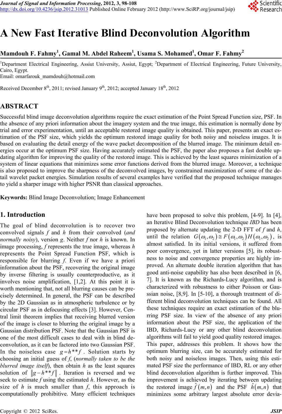
 Journal of Signal and Information Processing, 2012, 3, 98-108 http://dx.doi.org/10.4236/jsip.2012.31013 Published Online February 2012 (http://www.SciRP.org/journal/jsip) A New Fast Iterative Blind Deconvolution Algorithm Mamdouh F. Fahmy1, Gamal M. Abdel Raheem1, Usama S. Mohamed1, Omar F. Fahmy2 1Department Electrical Engineering, Assiut University, Assiut, Egypt; 2Department of Electrical Engineering, Future University, Cairo, Egypt. Email: omarfarouk_mamdouh@hotmail.com Received December 8th, 2011; revised January 9th, 2012; accepted January 18th, 2012 ABSTRACT Successful blind image deconvolution algorithms require the exact estimation of the Point Spread Function size, PSF. In the absence of any priori information about the imagery system and the true image, this estimation is normally done by trial and error experimentation, until an acceptable restored image quality is obtained. This paper, presents an exact es- timation of the PSF size, which yields the optimum restored image quality for both noisy and noiseless images. It is based on evaluating the detail energy of the wave packet decomposition of the blurred image. The minimum detail en- ergies occur at the optimum PSF size. Having accurately estimated the PSF, the paper also proposes a fast double up- dating algorithm for improving the quality of the restored image. This is achieved by the least squares minimization of a system of linear equations that minimizes some error functions derived from the blurred image. Moreover, a technique is also proposed to improve the sharpness of the deconvolved images, by constrained maximization of some of the de- tail wavelet packet energies. Simulation results of several examples have verified that the proposed technique manages to yield a sharper image with higher PSNR than classical approaches. Keywords: Blind Image Deconvolution; Image Enhancement 1. Introduction The goal of blind deconvolution is to recover two convolved signals f and h from their convolved (and normally noisy), version g. Neither f nor h is known. In image processing, f represents the true image, whereas h represents the Point Spread Function PSF, which is responsible for blurring f. Even if we have a priori information about the PSF, recovering the original image by inverse filtering is usually counterproductive, as it involves noise amplification, [1,2]. At this point it is worth mentioning that, not all blurring causes can be pre- cisely determined. In general, the PSF can be described by the 2D Gaussian as in atmospheric turbulence or by circular PSF as in defocusing effects [3]. However, Cen- tral limit theorem implies that receiving blurred version of the image is closer to blurring the original image by a Gaussian distribution PSF. Note that the Gaussian PSF is one of the most difficult cases to deal with in blind de- convolution, as it can be factored into two Gaussian PSF. In the noiseless case ** hf. Solution starts by choosing an initial guess of f, (normally taken to be the blurred image itself), then obtain h as the least squares solution of ** hf. Iteration is reversed and we seek to estimate f using the estimated h. However, as the size of h is much smaller than f, this approach is computationally prohibitive. Many efficient techniques have been proposed to solve this problem, [4-9]. In [4], an Iterative Blind Deconvolution technique IBD has been proposed by alternate updating the 2-D FFT of f and h, until the relation ,,GFH , 1212 12 , is almost satisfied. In its initial versions, it suffered from poor convergence, yet in latter versions [5], its robust- ness to noise and convergence properties are highly im- proved. An alternate double iteration algorithm that has good anti-noise capability has also been described in [6, 7]. It is known as the Richards-Lucy algorithm, and is characterized with robustness to either Poisson or Gau- ssian noise, [8,9]. In [5-10], a thorough treatment of di- fferent blind deconvolution techniques can be found. All these techniques require an exact estimation of the blu- rring PSF size. In view of the absence of any priori information about the PSF size, the application of the IBD, Richards-Lucy or any other blind deconvolution algorithms will fail to yield good quality restored images. This paper, addresses this problem. It shows how the optimum blurring size, can be accurately estimated for both noisy and noiseless images. Then, using this esti- mated PSF size the performance of IBD, RL or any other blind deconvolution algorithm is further improved. This improvement is achieved by iterating between updating the restored image ˆ, mn and the PSF ˆ,hmn that minimizes some arbitrary largest absolute error devia- Copyright © 2012 SciRes. JSIP 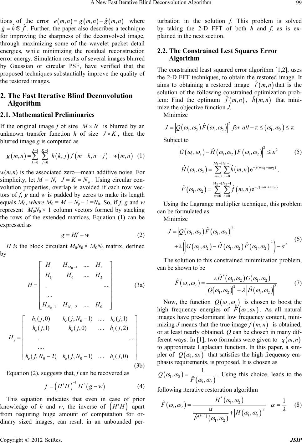 A New Fast Iterative Blind Deconvolution Algorithm 99 tions of the error where ˆ ,,emngmn gmn , ˆˆ ˆ hf. Further, the paper also describes a technique for improving the sharpness of the deconvolved image, through maximizing some of the wavelet packet detail energies, while minimizing the residual reconstruction error energy. Simulation results of several images blurred by Gaussian or circular PSF, have verified that the proposed techniques substantially improve the quality of the restored images. 2. The Fast Iterative Blind Deconvolution Algorithm 2.1. Mathematical Preliminaries If the original image f of size N is blurred by an unknown transfer function h of size K, then the blurred image g is computed as 11 00 ,,,, JK kj g hkjfmknmn mnjw (1) w(m,n) is the associated zero—mean additive noise. For simplicity, let M = N, KN . Using circular con- volution properties, overlap is avoided if each row vec- tors of f, g and w is padded by zeros to make its length equals M0, where M0 = M + Np – 1=N0. So, if f, g and w represent M0N0 × 1 column vectors formed by stacking the rows of the extended matrices, Equation (1) can be expressed as Hf w (2) H is the block circulant M0N0 × M0N0 matrix, defined by 0 1 00 011 10 2 12 0 .... .... .... . .... .... M NN HH H HH H H HH H (3a) 0 00 (,0)(,1) ....(,1) (,1)(,0).... (,2) . .... .... (,2)(,1)....(,0) ee e ee e j ee e hj hjNhj hj hjhj H hjN hjNhj (3b) Equation (2), suggests that, f can be recovered as 1 tt HHH g w (4) This equation indicates that even in case of prior knowledge of h and w, the inverse of t H apart from requiring huge amount of computation for or- dinary sized images, can result in an unbounded per- turbation in the solution f. This problem is solved by taking the 2-D FFT of both h and f, as is ex- plained in the next section. 2.2. The Constrained Lest Squares Error Algorithm The constrained least squared error algorithm [1,2], uses the 2-D FFT techniques, to obtain the restored image. It aims to obtaining a restored image ˆ, mn that is the solution of the following constrained optimization prob- lem: Find the optimum ˆ, mn , that mini- mize the objective function J, ˆ, hmn Minimize 2 12 1212 ˆ ,, π,πJQFfor all Subject to 22 121212 ˆ ,,,HGF (5) 11 12 11 () 12 00 ˆ ,,e ˆMN jm n mn nHhm , 22 12 11 () 12 00 ˆ ˆ,,e MN jm n mn Ffmn Using the Lagrange multiplier technique, this problem can be formulated as Minimize 2 12 12 22 1212 12 ˆ ,, ˆ ,ˆ,,H JQ F GF (6) The solution to this constrained minimization problem, can be shown to be * 12 12 12 2 2 12 12 ,, ˆ, ˆ ˆ ,, G FQ H H (7) Now, the function 12 ,Q ˆ F is chosen to boost the high frequency energies of 12 , , . As all natural images have pre-dominant low frequency content, mini- mizing J means that the true image mn is obtained, or at least nearly obtained. Q can be chosen in many dif- ferent ways. In [1], two formulas were given to ,qmn to approximate Laplacian function. In this paper, a sim- pler of 12 ,Q that satisfies the high frequency em- phasis requirements, is proposed. It is chosen as 12 12 1 ,ˆ, QF . Using this choice, leads to the following iterative restoration algorithm * 12 12 2 12 1 12 ,1 ˆ, , ˆ, k H FH F (8) Copyright © 2012 SciRes. JSIP 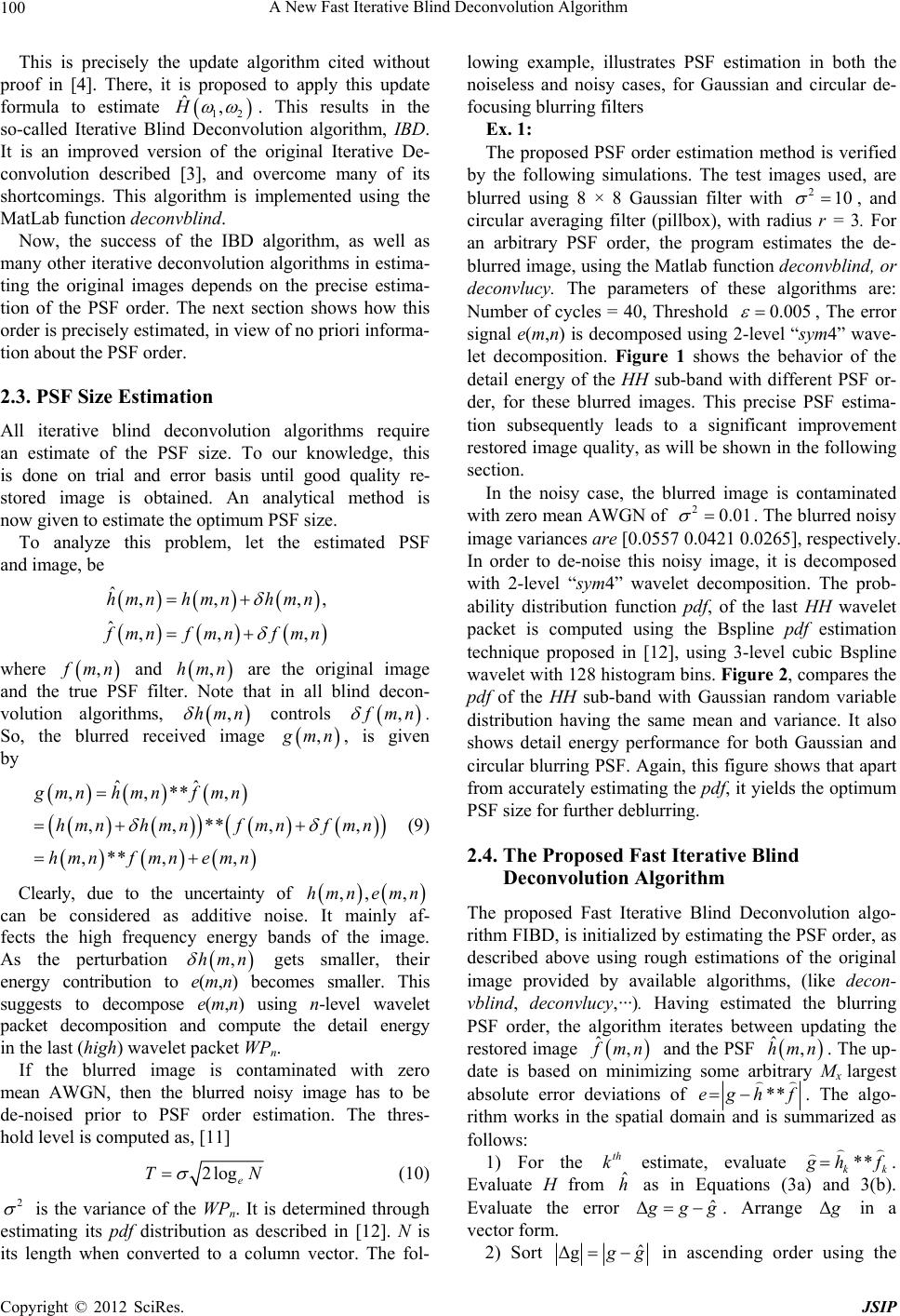 A New Fast Iterative Blind Deconvolution Algorithm 100 This is precisely the update algorithm cited without proof in [4]. There, it is proposed to apply this update formula to estimate 12 ˆ,H . This results in the so-called Iterative Blind Deconvolution algorithm, IBD. It is an improved version of the original Iterative De- convolution described [3], and overcome many of its shortcomings. This algorithm is implemented using the MatLab function deconvblind. Now, the success of the IBD algorithm, as well as many other iterative deconvolution algorithms in estima- ting the original images depends on the precise estima- tion of the PSF order. The next section shows how this order is precisely estimated, in view of no priori informa- tion about the PSF order. 2.3. PSF Size Estimation All iterative blind deconvolution algorithms require an estimate of the PSF size. To our knowledge, this is done on trial and error basis until good quality re- stored image is obtained. An analytical method is now given to estimate the optimum PSF size. To analyze this problem, let the estimated PSF and image, be ˆ,, , ˆ,, hmn hmnhmn, , mnfmnf mn where , mn and are the original image and the true PSF filter. Note that in all blind decon- volution algorithms, controls ,hmn ,hm n , mn . So, the blurred received image , mn , is given by ˆˆ ,,**, ,,**, ,** ,, gmnhmnf mn hmnhmnf mnf mn hmnf mnemn , (9) Clearly, due to the uncertainty of ,, ,hmn emn can be considered as additive noise. It mainly af- fects the high frequency energy bands of the image. As the perturbation gets smaller, their energy contribution to e(m,n) becomes smaller. This suggests to decompose e(m,n) using n-level wavelet packet decomposition and compute the detail energy in the last (high) wavelet packet WPn. ,hmn If the blurred image is contaminated with zero mean AWGN, then the blurred noisy image has to be de-noised prior to PSF order estimation. The thres- hold level is computed as, [11] 2loge T N (10) 2 is the variance of the WPn. It is determined through estimating its pdf distribution as described in [12]. N is its length when converted to a column vector. The fol- lowing example, illustrates PSF estimation in both the noiseless and noisy cases, for Gaussian and circular de- focusing blurring filters Ex. 1: The proposed PSF order estimation method is verified by the following simulations. The test images used, are blurred using 8 × 8 Gaussian filter with 210 , and circular averaging filter (pillbox), with radius r = 3. For an arbitrary PSF order, the program estimates the de- blurred image, using the Matlab function deconvblind, or deconvlucy. The parameters of these algorithms are: Number of cycles = 40, Threshold 0.005 , The error signal e(m,n) is decomposed using 2-level “sym4” wave- let decomposition. Figure 1 shows the behavior of the detail energy of the HH sub-band with different PSF or- der, for these blurred images. This precise PSF estima- tion subsequently leads to a significant improvement restored image quality, as will be shown in the following section. In the noisy case, the blurred image is contaminated with zero mean AWGN of . The blurred noisy image variances are [0.0557 0.0421 0.0265], respectively. In order to de-noise this noisy image, it is decomposed with 2-level “sym4” wavelet decomposition. The prob- ability distribution function pdf, of the last HH wavelet packet is computed using the Bspline pdf estimation technique proposed in [12], using 3-level cubic Bspline wavelet with 128 histogram bins. Figure 2, compares the pdf of the HH sub-band with Gaussian random variable distribution having the same mean and variance. It also shows detail energy performance for both Gaussian and circular blurring PSF. Again, this figure shows that apart from accurately estimating the pdf, it yields the optimum PSF size for further deblurring. 20.01 2.4. The Proposed Fast Iterative Blind Deconvolution Algorithm The proposed Fast Iterative Blind Deconvolution algo- rithm FIBD, is initialized by estimating the PSF order, as described above using rough estimations of the original image provided by available algorithms, (like decon- vblind, deconvlucy,···). Having estimated the blurring PSF order, the algorithm iterates between updating the restored image ˆ, mn and the PSF . The up- date is based on minimizing some arbitrary Mx largest absolute error deviations of ˆ,hmn **h feg . The algo- rithm works in the spatial domain and is summarized as follows: 1) For the estimate, evaluate th k** kk hf . Evaluate H from as in Equations (3a) and 3(b). Evaluate the error ˆ h ˆ Δ gg . Arrange Δ in a vector form. 2) Sort ˆ Δg g in ascending order using the Copyright © 2012 SciRes. JSIP 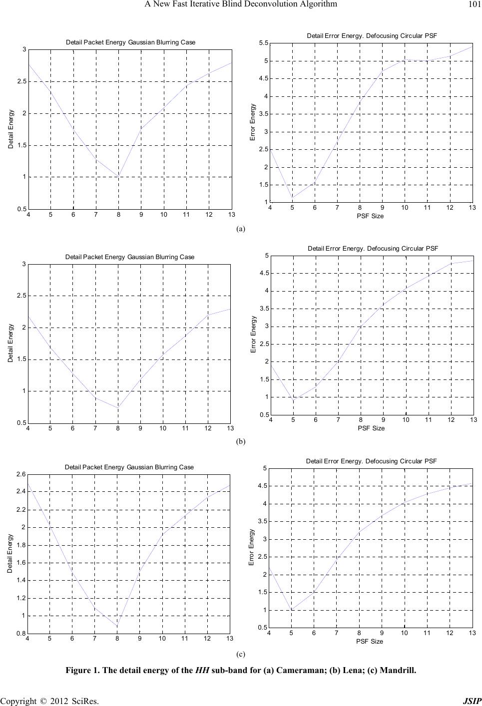 A New Fast Iterative Blind Deconvolution Algorithm Copyright © 2012 SciRes. JSIP 101 45 6 7 8 910 11 12 13 0.5 1 1.5 2 2.5 3Detail Pac ket Energy Gaussi an Blurring Case Deta il E nergy 45678910 11 12 13 1 1.5 2 2.5 3 3.5 4 4.5 5 5.5 PSF Size Error Energy Detail Error Energy. Defocusing Circular PSF (a) 45 6 78 910 11 1213 0.5 1 1.5 2 2.5 3Detail Pac ket Energy Gaussian Blurring Case Det a il En ergy 45 6 78 910 11 12 13 0.5 1 1.5 2 2.5 3 3.5 4 4.5 5 PSF Size Error Energy Detail Error Energy. Defocusing Circ ular PSF (b) 456789101112 13 0.8 1 1.2 1.4 1.6 1.8 2 2.2 2.4 2.6 D etail Pac ket Energy Gaussi an Blurri ng Case Deta il En ergy 4567891011 12 13 0.5 1 1.5 2 2.5 3 3.5 4 4.5 5 PSF Size Err or Energy Detail Error Energy. Def ocusing Circular PSF (c) Figure 1. The detail energy of the HH sub-band for (a) Cameraman; (b) Lena; (c) Mandrill. 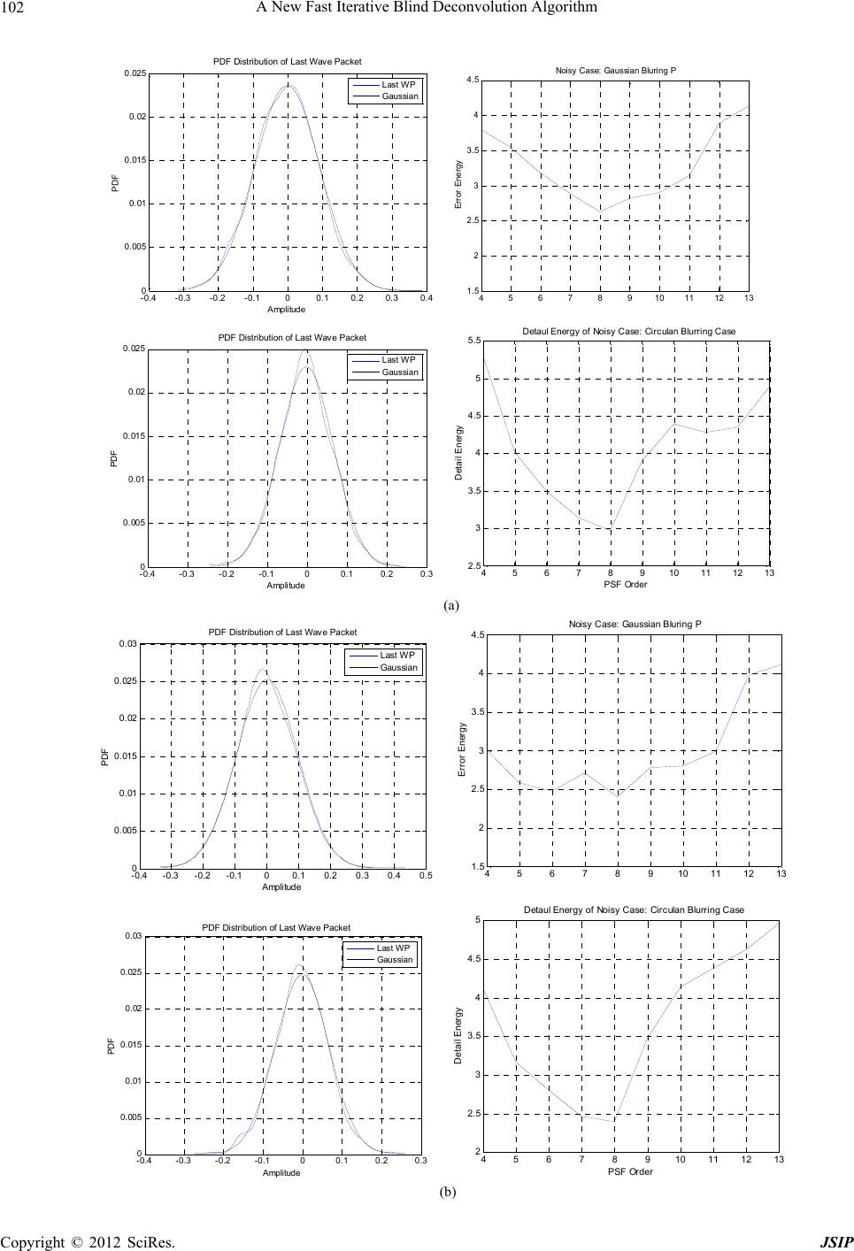 A New Fast Iterative Blind Deconvolution Algorithm 102 -0.4 -0.3 -0.2 -0.1 00.1 0.2 0.3 0.4 0 0.005 0.01 0.015 0.02 0.025 PDF dDstrubution of Last W ave Pac ket Amplitude PDF Last WP Gaussian PDF Distr ubution of Last Wave Pack et PDF Distribution of Last Wave Packet 45 6 7 8 910 111213 1.5 2 2.5 3 3.5 4 4.5 No isy Case : Gaussian Bl uring P Error Energy -0.4 -0.3 -0.2-0.1 00.1 0.2 0.3 0 0.005 0.01 0.015 0.02 0.025PDF dDstrubution of Last W ave Pac ket Amplitude PDF Last WP Gaussian PDF Distr ubution of Last Wave Packet PDF Distri bution of Last Wave Packet 45678910 11 12 13 2.5 3 3.5 4 4.5 5 5.5 Detail Energy PSF Order Detaul Energy of Noisy Case: Circulan Blurri ng Case (a) -0.4-0.3 -0.2 -0.100.1 0.2 0.3 0.4 0. 0 0.005 0.01 0.015 0.02 0.025 0.03 PDF dDstrubution of Last Wave Packet Amplitude PDF Last WP Gaussian PDF Distrubution of Last Wave Pac k et PDF Distr ibution of Last Wave Packet 45678910 11 12 13 1.5 2 2.5 3 3.5 4 4.5 Noisy Case : Gau ssian Bl uring P Error Energy -0.4 -0.3 -0.2 -0.1 00.1 0.2 0.3 0 0.005 0.01 0.015 0.02 0.025 0.03PDF dDstrubution of Last Wave Packet Amplitude PDF Last WP Gaussian PDF Distr ubution of Last Wave Pack et PDF Distr ibution of Last Wave Packe t 4567891011 12 13 2 2.5 3 3.5 4 4.5 5 Detail En ergy PSF Or der Detaul Energy of Noisy Case: Circ ulan Blurring Case (b) Copyright © 2012 SciRes. JSIP 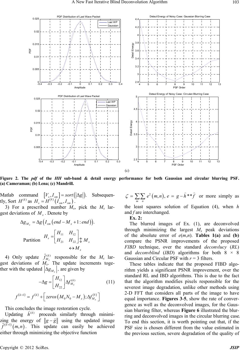 A New Fast Iterative Blind Deconvolution Algorithm Copyright © 2012 SciRes. JSIP 103 -0.4-0.3 -0.2-0.100.1 0.2 0.3 0.4 0 0.005 0.01 0.015 0.02 0.025 PDF dDstrubution of Last Wave Pack et Amplitude PDF Last WP Gaussia n PDF Distrubut ion of Last Wave Pack et PDF Distribution of Last Wave Packet 4567891011 1213 2.8 3 3.2 3.4 3.6 3.8 4 4.2 4.4 Detail Energy PSF Order Detaul E nergy of Noisy Case: Gaussian Blurri ng Case -0.4-0.3-0.2 -0.100.1 0.2 0.3 0 0.005 0.01 0.015 0.02 0.025PDF dDs t r ubution of Last Wave Packe t Amplitude PDF Last WP Gaussian PDF Distribution of Last Wave Pack et 4567891011 12 13 2.5 3 3.5 4 4.5 5 Detail En ergy PSF Order Detaul Energy of Noisy Case: Circulan Blurri ng Case (c) Figure 2. The pdf of the HH sub-band & detail energy performance for both Gaussian and circular blurring PSF. (a) Cameraman; (b) Lena; (c) Mandrill. Matlab command ,Δ xxm V Isortg . Subsequen- tly, Sort ()k as , k xm xm HII. 2,, ** mn emnegh f or more simply as the least squares solution of Equation (4), when h and f are interchanged. 3) For a prescribed number M x, pick the Mx lar- gest deviations of . Denote by ΔΔ 1: . x Mxm x g IendMend Ex. 2: The blurred images of Ex. (1), are deconvolved through minimizing the largest Mx peak deviations of the absolute error of e(m,n). Tables 1(a) and (b) compare the PSNR improvements of the proposed FIBD technique, over the standard deconvlucy (RL) and deconvblind (IBD) algorithms for both 8 × 8 Gaussian and Circular PSF with r = 3 filters. Partition 11 12 21 22 s x HH H HH M () ˆk 4) Only update x responsible for the M x lar- gest deviations of Mx. The update increments toge- ther with the updated Δx M , are given by 12 () 22 ΔΔ x k M H f H (11) 1 00 ;Δx k kk xM ffzerosM NMf These tables indicate that the proposed FIBD algo- rithm yields a significant PSNR improvement, over the standard RL and IBD algorithms. This is due to the fact that the algorithm modifies pixels responsible for the severest image degradation, unlike other methods using 2-D FFT that considers all parts of the image to have equal importance. Figures 3-5, show the rate of conver- gence as well as the deconvolved images, for the Gaus- sian blurring filter, whereas Figure 6 illustrated the blur- ring and deconvolved images in the circular blurring case. To end this section, it is worth pointing out that, if the PSF size is chosen different from the value estimated in the previous section, severe degradation of the quality of This concludes the image restoration cycle. Updating ()k h proceeds similarly through minimi- zing the energy of g using the updated image 1 ˆ, k mn . This update can easily be achieved either through minimizing the objective function 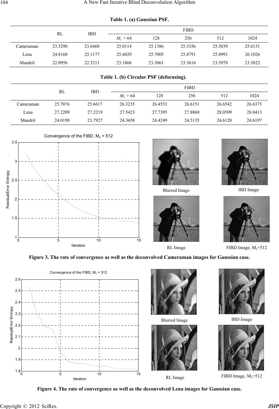 A New Fast Iterative Blind Deconvolution Algorithm 104 Table 1. (a) Gaussian PSF. FIBD RL IBD Mx = 64 128 256 512 1024 Cameraman 23.5290 23.6468 25.0114 25.1386 25.3356 25.5039 25.6131 Lena 24.8168 25.1177 25.6029 25.7005 25.8791 25.8991 26.1026 Mandril 22.0956 22.3211 23.1868 23.3061 23.3616 23.5978 23.5822 Table 1. (b) Circular PSF (defocusing). FIBD RL IBD Mx = 64 128 256 512 1024 Cameraman 25.7076 25.6617 26.3235 26.4553 26.6151 26.6542 26.6373 Lena 27.2209 27.2219 27.5423 27.7395 27.8868 28.0509 28.0413 Mandril 24.0190 23.7927 24.3658 24.4249 24.5135 24.6128 24.6197 05 10 15 1 1.5 2 2.5 3 3.5 Re sidu alError Entropy Iteration Convergence of the FIBD, M x =512 Convergence of the FIBD, M x = 512 Blurred ImageIBD Image RL ImageFIBD Image, M x =512 Figure 3. The rate of convergence as well as the deconvolved Cameraman images for Gaussian case. 05 10 15 1.8 1.9 2 2.1 2.2 2.3 2.4 2.5 2.6 Res idu alError Entropy Iteration Convergence of the FIBD, M x =512 Convergence of the FIBD, M x = 512 IBD Image Blurred Image RL Ima e FIBD Image, M x =512 Figure 4. The rate of convergence as well as the deconvolved Lena images for Gaussian case. Copyright © 2012 SciRes. JSIP 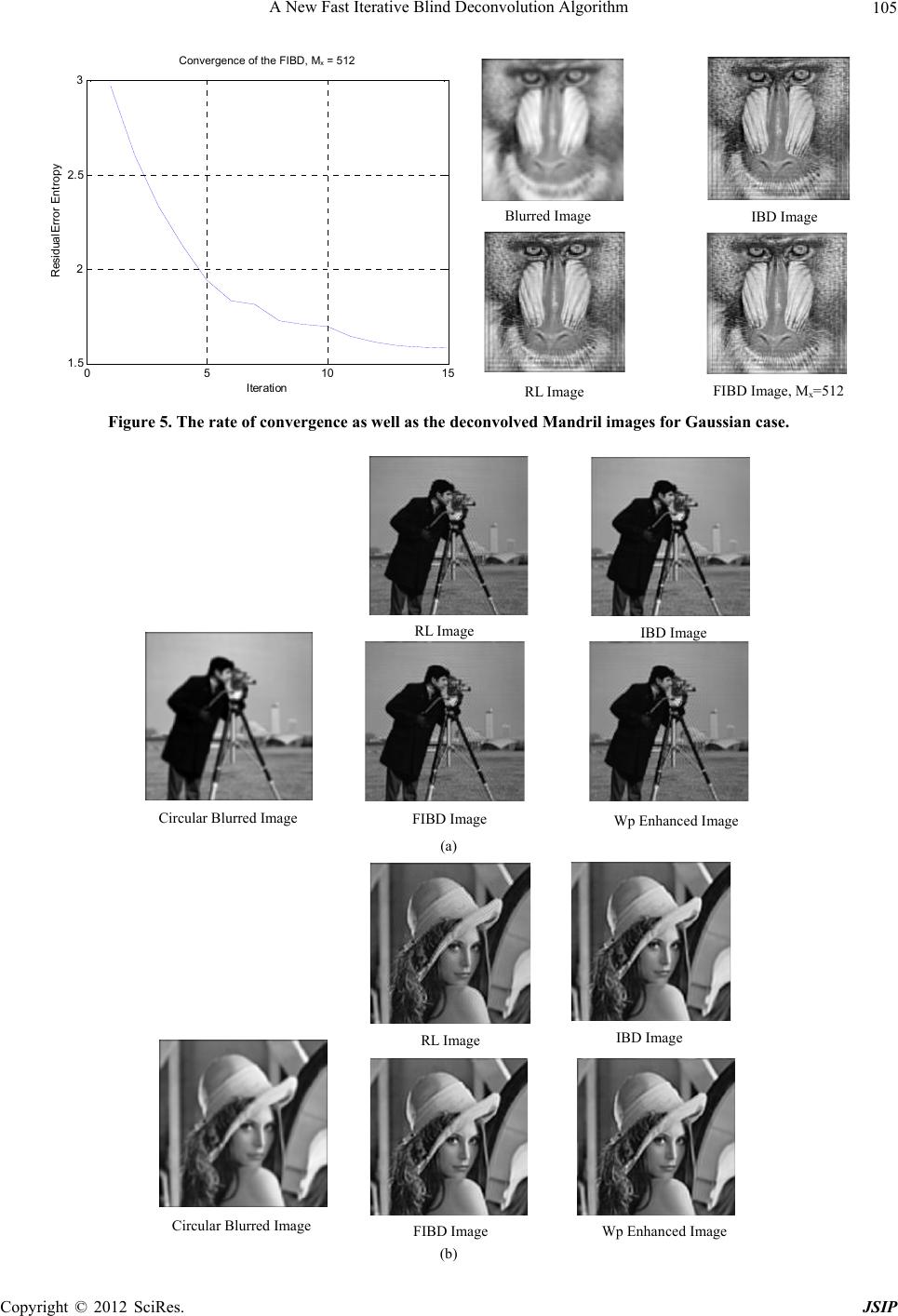 A New Fast Iterative Blind Deconvolution Algorithm 105 05 10 15 1.5 2 2.5 3 Re sidualEr ror Entropy Iter ation Convergence of the FIBD, M x =512 Converge nce of the FIBD, M x = 512 Blurred Image RL ImageFIBD Image, M x =512 IBD Image Figure 5. The rate of convergence as well as the deconvolved Mandril images for Gaussian case. Circular Blurred Image RL ImageIBD Image FIBD ImageWp Enhanced Image (a) Circular Blurred Image RL ImageIBD Image FIBD ImageWp Enhanced Image (b) Copyright © 2012 SciRes. JSIP 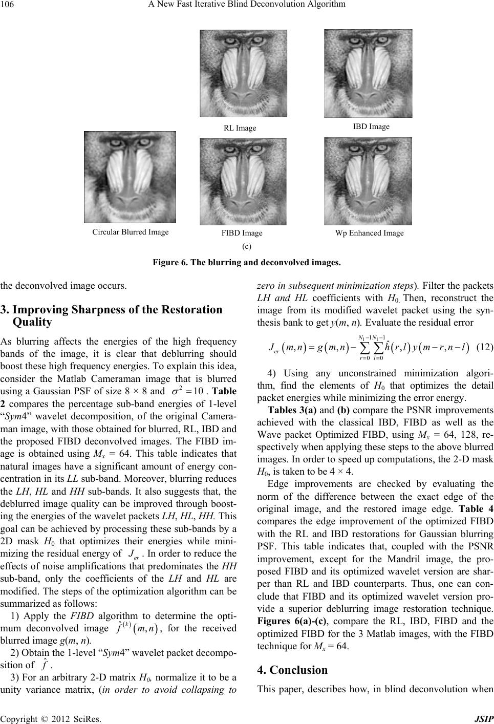 A New Fast Iterative Blind Deconvolution Algorithm Copyright © 2012 SciRes. JSIP 106 Circular Blurred Image RL ImageIBD Image FIBD ImageWp Enhanced Image (c) Figure 6. The blurring and deconvolved images. the deconvolved image occurs. 3. Improving Sharpness of the Restoration Quality As blurring affects the energies of the high frequency bands of the image, it is clear that deblurring should boost these high frequency energies. To explain this idea, consider the Matlab Cameraman image that is blurred using a Gaussian PSF of size 8 × 8 and . Table 2 compares the percentage sub-band energies of 1-level “Sym4” wavelet decomposition, of the original Camera- man image, with those obtained for blurred, RL, IBD and the proposed FIBD deconvolved images. The FIBD im- age is obtained using Mx = 64. This table indicates that natural images have a significant amount of energy con- centration in its LL sub-band. Moreover, blurring reduces the LH, HL and HH sub-bands. It also suggests that, the deblurred image quality can be improved through boost- ing the energies of the wavelet packets LH, HL, HH. This goal can be achieved by processing these sub-bands by a 2D mask H0 that optimizes their energies while mini- mizing the residual energy of er 210 . In order to reduce the effects of noise amplifications that predominates the HH sub-band, only the coefficients of the LH and HL are modified. The steps of the optimization algorithm can be summarized as follows: 1) Apply the FIBD algorithm to determine the opti- mum deconvolved image ˆ, k mn , for the received blurred image g(m, n). 2) Obtain the 1-level “Sym4” wavelet packet decompo- sition of ˆ . 3) For an arbitrary 2-D matrix H0, normalize it to be a unity variance matrix, (in order to avoid collapsing to zero in subsequent minimization steps). Filter the packets LH and HL coefficients with H0. Then, reconstruct the image from its modified wavelet packet using the syn- thesis bank to get y(m, n). Evaluate the residual error 11 11 00 ˆ ,,, , NN er rl mngmnhrlymrnl (12) 4) Using any unconstrained minimization algori- thm, find the elements of H0 that optimizes the detail packet energies while minimizing the error energy. Tables 3(a) and (b) compare the PSNR improvements achieved with the classical IBD, FIBD as well as the Wave packet Optimized FIBD, using Mx = 64, 128, re- spectively when applying these steps to the above blurred images. In order to speed up computations, the 2-D mask H0, is taken to be 4 × 4. Edge improvements are checked by evaluating the norm of the difference between the exact edge of the original image, and the restored image edge. Table 4 compares the edge improvement of the optimized FIBD with the RL and IBD restorations for Gaussian blurring PSF. This table indicates that, coupled with the PSNR improvement, except for the Mandril image, the pro- posed FIBD and its optimized wavelet version are shar- per than RL and IBD counterparts. Thus, one can con- clude that FIBD and its optimized wavelet version pro- vide a superior deblurring image restoration technique. Figures 6(a)-(c), compare the RL, IBD, FIBD and the optimized FIBD for the 3 Matlab images, with the FIBD technique for Mx = 64. 4. Conclusion This paper, describes how, in blind deconvolution when 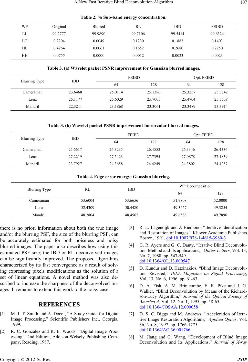 A New Fast Iterative Blind Deconvolution Algorithm 107 Table 2. % Sub-band energy conce ntration. WP Original Blurred RL IBD FEIBD LL 99.2777 99.9890 99.7106 99.5414 99.6324 LH 0.2204 0.0049 0.1230 0.1883 0.1403 HL 0.4264 0.0061 0.1652 0.2680 0.2250 HH 0.0755 0.0000 0.0012 0.0023 0.0023 Table 3. (a) Wavelet packet PSNR improvement for Gaussian blurred images. FEIBD Opt. FEIBD Blurring Type IBD 64 128 64 128 Cameraman 23.6468 25.0114 25.1386 25.3257 25.3742 Lena 25.1177 25.6029 25.7005 25.4704 25.5538 Mandril 22,3211 23.1868 23.3061 23.3489 23.3914 Table 3. (b) Wavelet packet PSNR improvement for circular blurred images. FEIBD Opt. FEIBD Blurring Type IBD 64 128 64 128 Cameraman 25.6617 26.3235 26.4553 26.3346 26.4336 Lena 27.2219 27.5423 27.7395 27.0878 27.1839 Mandril 23.7927 24.3658 24.4249 24.3802 24.4237 Table 4. Edge error energy: Gaussian blurring. WP Decomposition Blurring Type RL IBD 64 128 Cameraman 53.6004 53.6656 51.9808 52.0000 Lena 52.4309 50.4480 49.3457 49.3254 Mandril 48.2804 48.4562 49.6588 49.7896 there is no priori information about both the true image and/or the blurring PSF, the size of the blurring PSF, can be accurately estimated for both noiseless and noisy blurred images. The paper also describes how using this estimated PSF size; the IBD or RL deconvolved images can be significantly improved. The proposed algorithms characterized by its fast convergence as a result of solv- ing expressing pixels modifications as the solution of a set of linear equations. A novel method was also de- scribed to increase the sharpness of the deconvolved im- ages. It remains to extend this work to the noisy case. REFERENCES [1] M. J. T. Smith and A. Docef, “A Study Guide for Digital Image Processing,” Scientific Publishers Inc., Georgia, 1999. [2] R. C. Gonzalez and R. E. Woods, “Digital Image Proc- essing,” 2nd Edition, Addison-Welsely Publishing Com- pany, Reading, 1987. [3] R. L. Lagendijk and J. Biemond, “Iterative Identification and Restoration of Images,” Kluwer Academic Publishers, Boston, 1991. doi:10.1007/978-1-4615-3980-3 [4] G. R. Ayers and G. C. Danty, “Ierative Blind Deconvolu- tion Method and Its applications,” Optics Letters, Vol. 13, No. 7, 1988, pp. 547-549. doi:10.1364/OL.13.000547 [5] D. Kundur and D. Hatzinakios, “Blind Image Deconvolu- tion Revisted,” IEEE Magazine on Signal Processing, Vol. 13, No. 6, 1996, pp. 61-63. [6] D. A. Fish, A. M. Brinicombe, E. R. Pike and J. G. Walker, “Blind Deconvolution by Means of the Richard- son-Lucy Algorithm,” Journal of the Optical Society of America A, Vol. 12, No. 1, 1995, pp. 58-65. doi:10.1364/JOSAA.12.000058 [7] D. S. C. Biggs and M. Andrews, “Acceleration of Itera- tive Image Restoration Algorithms,” Applied Optics, Vol. 36, No. 8, 1997, pp. 1766-1775. doi:10.1364/AO.36.001766 [8] M. Jiang and G. Wang, “Development of Blind Image Deconvolution and Its Applications,” Journal of X-ray Copyright © 2012 SciRes. JSIP  A New Fast Iterative Blind Deconvolution Algorithm 108 Science and Ology, Vol. 11, 2003, pp. 13-19. [9] H. Y. Liu, Y. S. Zhang and J. I. Song, “Study on the Methods of Super Resolution Image Reconstruction,” The International Archives of the Photognanmetry, Remote Sensing and Spatial Information Science, Vol. XXVII, Part B2, Beijing, 2008. [10] D. Kundur and D. Hatzinakios, “Blind Image Deconvo- lution,” IEEE Magazine on Signal Processing, Vol. 13, No. 3, 1996, pp. 43-64. [11] S. Mallat, “A Wavelet Tour of Signal Processing, the Sparse Way,” Academic Press, New York, 2009. [12] M. F. Fahmy, G. M. Fahmy and O. M. Fahmy, “Bspline Wavelets in Signal De-Noising and Image Compression,” Journal of Signal, Image and Video Processing, Vol. 5, No. 2, 2011, pp. 141-153. doi:10.1007/s11760-009-0148-x Copyright © 2012 SciRes. JSIP
|