Journal of Mathematical Finance, 2012, 2, 121-131
http://dx.doi.org/10.4236/jmf.2012.21014 Published Online February 2012 (http://www.SciRP.org/journal/jmf)
Forecasting Volatility of Gold Price Using Markov Regime
Switching and Trading Strategy
Nop Sopipan1, Pairote Sattayatham1, Bhusana Premanode2
1School of Mathematics Suranaree, University of Technology, Nakhon Ratchasima, Thailand
2Institute of Biomedical Engineering, Imperial College South Kensington Campus, London, UK
Received October 24, 2011; revised December 1, 2011; accepted December 15, 2011
ABSTRACT
In this paper, we forecast the volatility of gold prices using Markov Regime Switching GARCH (MRS-GARCH) mod-
els. These models allow volatility to have different dynamics according to unobserved regime variables. The main pur-
pose of this paper is to find out whether MRS-GARCH models are an improvement on the GARCH type models in
terms of modeling and forecasting gold price volatility. The MRS-GARCH is best performance model for gold price
volatility in some loss function. Moreover, we forecast closing prices of gold price to trade future contract. MRS-
GARCH got the most cumulative return same GJR model.
Keywords: Forecasting; Volatility; Gold Price; Markov Regime Switching
1. Introduction
The characteristic that all financial markets have in com-
mon is uncertainty, which is related to their short and long-
term price state. This feature is undesirable for the investor
but it is also unavoidable whenever the financial market
is selected as the investment tool. The best that one can
do is to try to reduce this uncertainty. Financial market
forecasting (or Prediction) is one of the instruments in
this process.
The financial market forecasting task divides researchers
and academics into two groups: those who believe that
we can devise mechanisms to predict the market and
those who believe that the market is efficient and when-
ever new information comes up the market absorbs it by
correcting itself, thus there is no space for prediction. Fur-
thermore they believe that the financial market follows a
random walk, which implies that the best prediction you
can have about tomorrow’s value is today’s value.
In time series, a financial price transformated to log
return series for stationary process which look like white
noise. Mehmet [1] said financial returns have three
characteristics. First is volatility clustering that means
large changes tend to be followed by large changes and
small changes tend to be followed by small changes.
Second is fat tailedness (excess kurtosis) which means
that financial returns often display a fatter tail than a
standard normal distribution and the third is leverage
effect which means that negative returns result in higher
volatility than positive returns of the same size.
The generalized autoregressive conditional heteroske-
dasticity (GARCH) models mainly capture three charac-
teristics of financial returns. The development of GARCH
type models was started by Engle [2]. Engle introduced
ARCH to model the heteroskedasticity by relating the
conditional variance of the disturbance term to the linear
combination of the squared disturbances in the recent past.
Bollerslev [3] generalized the ARCH (GARCH) model by
modeling the conditional variance to depend on its lagged
values as well as squared lagged values of disturbance.
The Exponential GARCH (EGARCH) model proposed
by Nelson [4] to cope with the skewness of ten encoun-
tered in financial returns, led to GJR-GARCH which was
introduced independently by Glosten, Aganathan, and
Runkle [5] to account for the leverage effect.
Hamilton and Susmel [6] stated that the spurious high
persistence problem in GARCH type models can be
solved by combining the Markov Regime Switching (MRS)
model with ARCH models (SWARCH). The idea behind
regime switching models is that as market conditions
change, the factors that influence volatility also change.
Nowaday some researchers have development of GARCH
model, as well as the benefit of using GARCH model [1,
7-9].
Gold is a precious metal which is also classed as a
commodity and a monetary asset. Gold has acted as a mul-
tifaceted metal through the centuries, possessing similar
characteristics to money in that it acts as a store of wealth,
a medium of exchange and a unit of value. Gold has also
played an important role as a precious metal with sig-
C
opyright © 2012 SciRes. JMF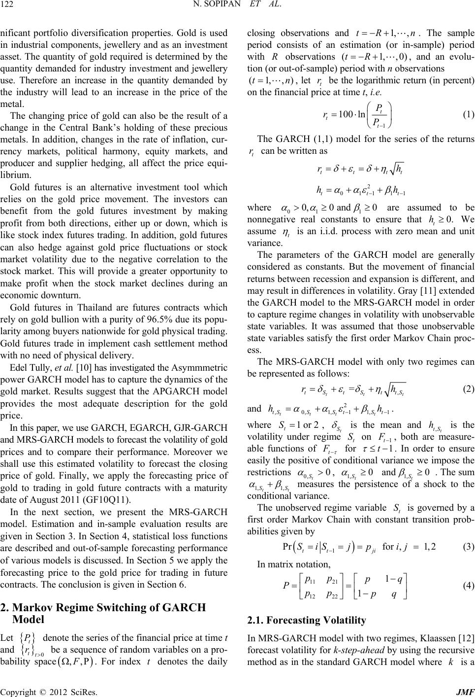

N. SOPIPAN ET AL. 122
nificant portfolio diversification properties. Gold is used
in industrial components, jewellery and as an investment
asset. The quantity of gold required is determined by the
quantity demanded for industry investment and jewellery
use. Therefore an increase in the quantity demanded by
the industry will lead to an increase in the price of the
metal.
The changing price of gold can also be the result of a
change in the Central Bank’s holding of these precious
metals. In addition, changes in the rate of inflation, cur-
rency markets, political harmony, equity markets, and
producer and supplier hedging, all affect the price equi-
librium.
Gold futures is an alternative investment tool which
relies on the gold price movement. The investors can
benefit from the gold futures investment by making
profit from both directions, either up or down, which is
like stock index futures trading. In addition, gold futures
can also hedge against gold price fluctuations or stock
market volatility due to the negative correlation to the
stock market. This will provide a greater opportunity to
make profit when the stock market declines during an
economic downturn.
Gold futures in Thailand are futures contracts which
rely on gold bullion with a purity of 96.5% due its popu-
larity among buyers nationwide for gold physical trading.
Gold futures trade in implement cash settlement method
with no need of physical delivery.
Edel Tully, et al. [10] has investigated the Asymmmetric
power GARCH model has to capture the dynamics of the
gold market. Results suggest that the APGARCH model
provides the most adequate description for the gold
price.
In this paper, we use GARCH, EGARCH, GJR-GARCH
and MRS-GARCH models to forecast the volatility of gold
prices and to compare their performance. Moreover we
shall use this estimated volatility to forecast the closing
price of gold. Finally, we apply the forecasting price of
gold to trading in gold future contracts with a maturity
date of August 2011 (GF10Q11).
In the next section, we present the MRS-GARCH
model. Estimation and in-sample evaluation results are
given in Section 3. In Section 4, statistical loss functions
are described and out-of-sample forecasting performance
of various models is discussed. In Section 5 we apply the
forecasting price to the gold price for trading in future
contracts. The conclusion is given in Section 6.
2. Markov Regime Switching of GARCH
Model
Let denote the series of the financial price at time t
and

0
tt
rbe a sequence of random variables on a pro-
bability space

,F index t den tes the daily
closing observations and tR sample
period consists of an estimation (or in-sample) period
with R obseations (tR

t
P

,. Foro
n. The
rv )
1, ,
1,,0

n evolu-
tion (or out-of-sample) period with n observations
, and a
)(1,tn,

, let t be the logarithmic return (in percent)
on the financial price at time t, i.e.
r
1
100 lnt
t
P
P




t
r (1)
The GARCH (1,1) model for the series of the returns
can be written as
t
r
ttt
rh    t
1t
2
0111tt
hh  


where 01 1 0,0 and 0

  are assumed to be
nonnegative real constants to ensure th0.
t We
assume t
at h

is an i.i.d. process with zero mean and unit
variance.
The parameters of the GARCH model are generally
considered as constants. But the movement of financial
returns between recession and expansion is different, and
may result in differences in volatility. Gray [11] extended
the GARCH model to the MRS-GARCH model in order
to capture regime changes in volatility with unobservable
state variables. It was assumed that those unobservable
state variables satisfy the first order Markov Chain proc-
ess.
The MRS-GARCH model with only two regimes can
be represented as follows:
,
=
tt t
tSttS
rh   
1
tS
,

(2)
and 2
,01,11,
tttt
SS tS t
hh 
tS



2
.
where t1 orS

, t
S

is the mean and ,t
tS is the
volatility under regime t on h
S1t
F
, both are measure-
able functions of t
F


for 1t

. In order to ensure
easily the positive of conditional variance we impose the
restrictions t
0,S0

, 1, t
S0

 1, and t
S
0

. The sum
1, 1,
tt
SS



measures the persistence of a shock to the
conditional variance.
The unobserved regime variable t is governed by a
first order Markov Chain with constant transition prob-
abilities given by
S


1 for , 1,2 tt ji
SiSjpij

Pr
P
(3)
In matrix notation,
11 21
12 22
1
1
pp p
pp pq

 q









 (4)
2.1. Forecasting Volatility
In MRS-GARCH model with two regimes, Klaassen [12]
forecast volatility for k-step-ahead by using the recursive
method as in the standard GARCH model where is a k

N. SOPIPAN ET AL. 123
positive integer. In order to compute the multi-step-ahead
volatility forecasts, we firstly compute a weighted aver-
age of the multi-step-ahead volatility forecasts in each
regime where the weights are the prediction probability
(

1
Pr TT SiF
 
).
Since there is no serial correlation in the returns, the
k-step-ahead volatility forecast at time T depends on
information at time T − 1. Let

,TT k
h denote the time T
aggregated volatility forecasts for the next k steps. It can
be calculated as follows: (See, for example Marcucci [9],
page 8)



,,
1
2
,,
1
11
Pr .
T
k
TT kTT
k
TT Si
TT
i
h
iFh
h
S



















(5)
where

,,
T
TT Si
h




indicates the

-step-ahead volatile-
ity forecast in regime i made at time T and can be calcu-
lated recursively as follows:








,, 1
2
0,1,1 1
1, 1
2
0,1,1 111
1, 1
0,
1
1
1
1, 1,
=
=[]
=
T
TT
T
TT
T
TTT
T
T
T
TT siTT
SiSiT TT
SiT T
SiSiTT TTT
SiT T
SiSi SiT
Ei
Ei
Ei
EE Si
hhS
S
h
E
S
S
hi
E
S















 

 











 

 

 











1,1 . TT T
Sih
 

(6)
Also, in generally the prediction probability in (5) is
computed as

 
11
1
11
Pr1Pr 1
Pr2Pr 2
TT TT
TT TT
FFSS
P
FFSS


 

 


 









1
1
,
where P defined in (4) and

11
Pr will be
discussed in (11). Lastly, we compute expectation part
TT
SiF



1,1TTT T
EhS i
 


in (6) as follows:

1,11 1
2
11 1
2
11 11
2
11 11
2
11 11
,
=,
,,
=[,] ,
[,],
TTTTT TT
TT T
TTT TT
TTTT T
TTT TT
EhSiEh SiF
EEr SjF
Er SjFSiF
EErSjF SiF
EEr SjFSiF
 


 
 
 
 
 
 
 

 























where
(7)





2
11 11
22
11 1
1
11
22
11 11
1
11
22
1111
[
TT
EEr


,],
,
Pr,
,
Pr,
2
TT T
TT T
j
TTT
TT TT
j
TTT
TTTT
SjFSiF
Er SjF
SjSiF
ESjF
SjSiF
E
 


 




 
 

 
 

 
 







 



 









11
2
11
1
11
22
, 11,1,
1
,
Pr,
=TT
TT
j
TTT
jiTT SjT Sj
j
SjF
SjSiF
ph





 
 

 
  














(8)
where




,1 11
11
1
Pr ,
Pr
Pr
ji TTTT
TT
TT
ji
SS
S
S
pj
pjF
iF




 




iF

. (9)
Similarly, we computed in the second term of right
hand side in (7) such that

1
2
11 1
22
1, ,1
1
1
,],
=T
TTT TT
TS j ji T
j
FSiF
p

 



 
  

[EEr Sj











 (10)
substitutes both (8) and (10) to (7) such that

11
1
,1
1()
TT
TT
22
, 11,1,
1
22
,1 1,
1
.
TT
T
j
iTT SjTSj
j
ji TTSj
j
ph
p






 

   

 

EhS i
 













In the next step, we will compute those regime prob-
abilities


1
Pr
ittt
pSiF

 for 1, 2i in (9). Note
that whenlities are based on informa-
tion up to time t, we describe this as filtered probability
(
the regime probabi


Pr tt SiF).
compute the regime probabilities, we de-
no
In order to
te


11
1:,
tttt
Sffr F

,


21
2:,
tttt
Sffr F

.
Then, n-
comes a mixture-of-distribution model in which mixing
variables is regime probability it p. That is
conditional distributio of return series be
t
r
1
(1,) witrobability
ttt
frSF1
1
121
h p
(2,) with probability 1,
t
tt
tt ttt
p
rF
f
rS Fpp







where





1
,
tt t
frSF
 denotes one of the assumed condi-

N. SOPIPAN ET AL. 124
tional dor errors: Normal Distribution (N),
Student-t Distribution with only single degree of freedom
(t) or double degree of freedom (2t) and Generalized er-
ror distributions (GED).
We shall compute reg
istributions f
ime probabilities recursively by
following two steps (Kim and Nelson, [13], page 63):
Step 1: Given

Pr SjF at the end of the ti
11tt me
probabilities 1, the regimet

Pr
it SiF are
uted as
1tt
p
comp

2
11
1
PrPr ,
tttt t
j
SiFSiS jF


 
1
.
Since the current regime) only depends on the re-
gi
(t
S
enme one period ago (1t S), th



1
2
111
1
2
11
1
Pr Pr
=Pr
tt t t
j
ji tt
j
Si jSSjF
pSjF
 




 



.
Step 2: At the end of the time t, when observed return
at
Pr tt SiF


time t (t
r) the information at time t set


1, ttt
F
Fr

,
the

Pr tt SiF is calculated as follows:



1
1
1
Pr Pr,= tt t
tt ttt
tt
iF
SiF SirFfrF



 ,
where
,frS

1
,
ttt
frS iF

 is joint density of returns and
rved regime at sunobsetate i for 1, 2i variables can
be written as follows:


111
11
,P
r
tt ttttt t
tttt t
frS iFfS iF
frSiFS iF


 
 
and
,,frS iF

1tt
frF
 is marginal density function of returns
e construccan bted as follows:
 

2
11
1
2
11
1
,
,Pr.
tttt t
i
tttt t
i
frFfrS iF
frSiFS iF





 


We use Bayesian arguments



 
 
1
1
11
2
11
1
2
1
,
Pr
,Pr
=
,Pr
=.
tt t
tt
tt
tt ttt
tt ttt
i
it it
it it
i
frS iF
SiF frF
frSiFS iF
frSiFS iF
fp
fp












(11)
Then, all regime probabilities can be computed by
iterating these two steps. Howe at the beginning of
iteration
it
p
ver,


00
Pr SiF for are necessary to
start iteration. Hamilton ([14,gest we should use
unconditional regime probabilof
1,
) su
ities instead
2i
15] g


00
Pr SiF. These are given by


100
200
1
πPr 1,
2
1
πPr 22
q
SF pq
p
SF pq






n and conditiorance
g-likeliursively
similar to that in
2.2. Forecasting Price
We forecast financial price at k-step-ahead with MRS-
GARCH models. Denote is k-step-ahead fore-
ca
Given initial values for regime probabilities, condi-
tional meanal va i in each regime, the
parameters of the MRS-GARCH model can be obtained
by maximizing numerically the log-likelihood function.
The lohood function is constructed rec
GARCH models
,
ˆ
tt k
r
sting logarithm return of financial price at time t de-
pend on 1t
F

.
We compute as:
 
2
,1 1,,
1
ˆˆ
Pr tk
ttkttktktttkSi
i
rEr SiFr


 

 
 (12)
where


,, 1
1
11
2
=
=
tk
tt
kk
ttk ttktk
ES
i
ESiE Si





 



11
1
2
,1
1
r ,
=
tk
tk
tk
t
tktktSi
j
Si ji t
j
i
SjSiF
p







 

 
ˆ
ttkSittk rErS
 
 

=P

  

 



Forecasting financial price one-step-ahead, we use (12)
and (1) combine in log-return of financial price is


1
22
11 ,1
11
1
Pr
ˆexp 100
t
tt jitS
ij
tt
SiF p
PP





i


 













. (3)
3. Empirical Methodology and Model
Estimation Results
3.
prices
of gold price
1
1. Data
The data set used in this study is the daily closed


t
P over the period 4/01/2007 through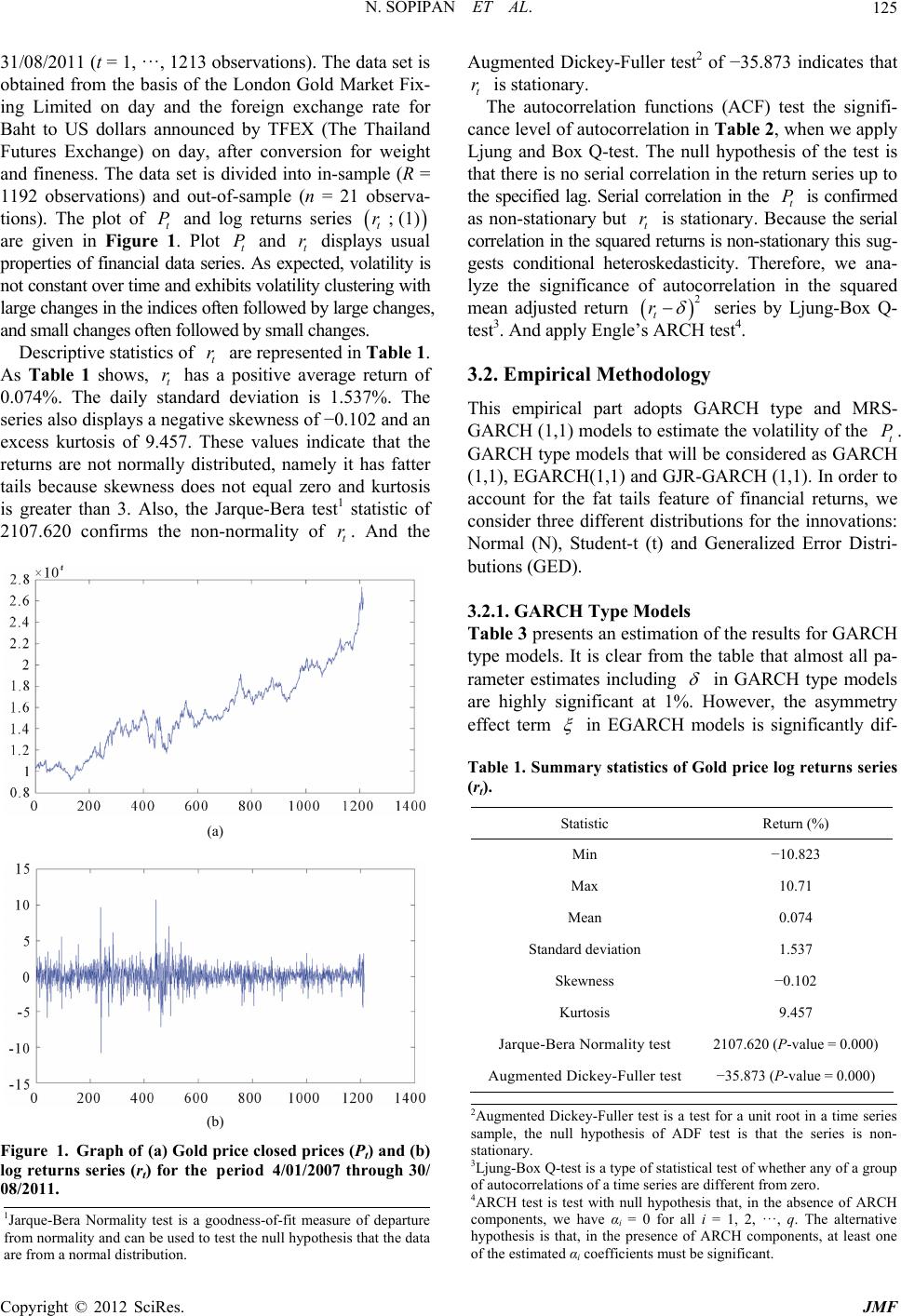

N. SOPIPAN ET AL. 125
31/08/2011 (t = 1, ···, 1213 observations). The data set is
obtained from the basis of the London Gold Market Fix-
ing Limited on day and the foreign exchange ra
Baht to US dollars announced by TFEX (The Thailand
Futures Exchange) on day, after conversion for weight
R =
serva-
tio log returns series
te for
and fineness. The data set is divided into in-sample (
1192 observations) and out-of-sample (n = 21 ob
ns). The plot of t
P and


; (1)
t
r
lays usual
, volatility is
kurtosis
are given i
properties of fi
n Figure . Plot and disp
na seexcted
the
1
ncial data
t
P
ries. As
t
r
pe
not constant over time and exhibits volatility clustering with
large changes inindices often followed by large changes,
and small changes often followed by small changes.
Descriptive statistics of t r are represented in Table 1.
As Table 1 shows, t r has a positive average return of
0.074%. The daily standard deviation is 1.537%. The
series also displays a negative skewness of −0.102 and an
excess kurtosis of 9.457. These values indicate that the
returns are not normally distributed, namely it has fatter
tails because skewness does not equal zero and
is greater than 3. Also, the Jarque-Bera test1 statistic of
2107.620 confirms the non-normality of t r. And the
(a)
Pt) and (b)
07 through 30/
(b)
Figure 1. Graph of plosedices (
log returns series (rtthe pd
08/2011.
Augmented Dickey-Fuller test2 of −35.873 indicates that
is stationary.
The autocorrelation functions (ACF) test the signifi-
cance level of autocorrelation in Table 2, when we apply
Ljung and Box Q-test. The null hypothesis of the test is
that there is no serial correlation in the return series up to
the specified lag. Serial correlation in the is confirmed
as non-stationary but is stationary. Because the serial
correlation in the squaeturns is non-stary this sug-
gests conditional heteroskedasticity. Therefre, we ana-
lyze the significance of autocorrelation in the square
mean adjusted return
(a) Gold
) for rice c erio pr 4/01/20
t
r
t
P
ation
o
t
r
red r
t
r
d

2

 series bg-Box Q-
ogy
G
imation
y Ljun
test3. And apply Engle’s ARCH test4.
3.2. Empirical Methodol
This empirical part adopts GARCH type and MRS-
ARCH (1,1) models to estimate the volatility of the t P.
GARCH type models that will be considered as GARCH
(1,1), EGARCH(1,1) and GJR-GARCH (1,1). In order to
account for the fat tails feature of financial returns, we
consider three different distributions for the innovations:
Normal (N), Student-t (t) and Generalized Error Distri-
butions (GED).
3.2.1. GARCH Type Models
Table 3 presents an estof the results for GARCH
type models. It is clear from the table that almost all pa-
rameter estimates including

in GARCH type models
wever, the asymmetry are highly significant at 1%. Ho
effect term

in EGARCH models is significantly dif-
ie Table 1. Summary statistics of Gold price log returns sers
(rt).
Statistic Return (%)
Min −10.823
Max 10.71
Mean 0.074
Standard deviation 1.537
Skewness −0.102
Kurtosis 9.457
Jarque-Bera Normality test 2107.620 (P-value = 0.000)
Augmented Dickey-Fuller test −35.873 (P-value = 0.000)
2Augmented Dickey-Fuller test is a test for a unit root in a time series
sample, the null hypothesis of ADF test is that the series is non-
stationary.
3Ljung-Box Q-test is a type of statistical test of whether any of a group
of autocorrelations of a time series are different from zero.
4ARCH test is test with null hypothesis that, in the absence of ARCH
components, we have αi = 0 for all i = 1, 2, ···, q. The alternative
hypothesis is that, in the presence of ARCH components, at least one
of the estimated αicoefficients must be significant.
1Jarque-Bera Normality test is a goodness-of-fit measure of departure
from normality and can be used to test the null hypothesis that the data
are from a normal distribution.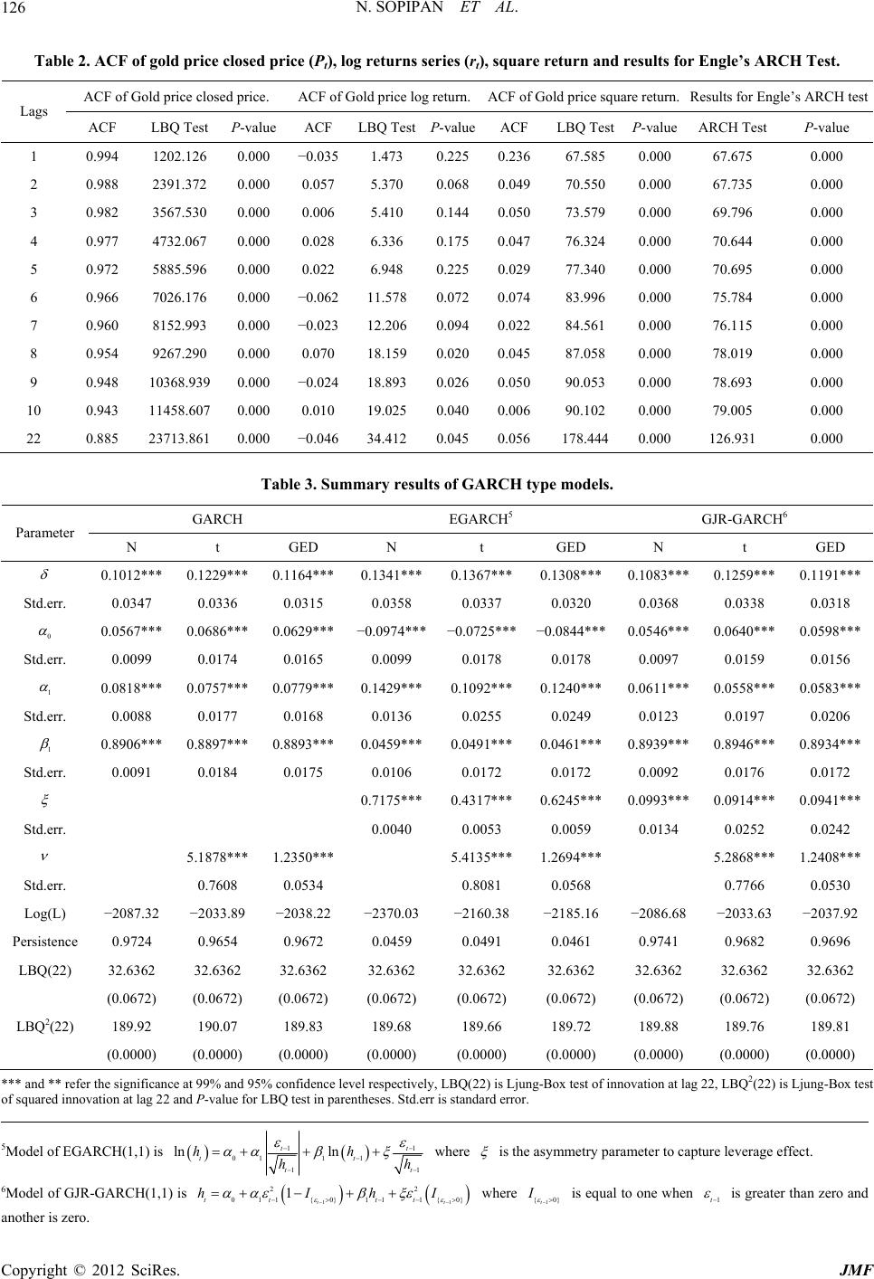

N. SOPIPAN ET AL. 126
eries (rt), squesults for Engle’s Test.
ACF of Gold price closed price. ACF of Gold price log return.ACF of quare return. Results for Engle’s ARCH test
Table 2. ACF of gold price closed price (Pt), log returns sare return and rARCH
Gold price s
Lags
ACF LBQ Test P-value ACF LBQ TestP-valueACF LBQ stP-value ARCH TeP-value Te st
1 0.994 1202.126 0.000 473 0.2250 −0.035 1.0.236 67.585 0.0067.675 0.000
2 0.988 2391.372 0.000 0.5.370 0.068
3 0.3567.530 0.000 5.410 0.1440.050 73.579 0.000 69.796 0.000
6 −
057 0.049 70.550 0.00067.735 0.000
982 0.006
4 0.977 4732.067 0.000 0.028 6.336 0.1750.047 76.324 0.000 70.644 0.000
5 0.972 5885.596 0.000 0.022 6.948 0.2250.029 77.340 0.000 70.695 0.000
0.966 7026.176 0.000 0.062 11.578 0.072 0.074 83.996 0.000 75.784 0.000
7 0.960 8152.993 0.000 −0.023 12.206 0.094 0.022 84.561 0.000 76.115 0.000
8 0.954 9267.290 0.000 0.070 18.159 0.0200.045 87.058 0.000 78.019 0.000
9 0.948 10368.939 0.000 −0.024 18.893 0.026 0.050 90.053 0.000 78.693 0.000
10 0.943 11458.607 0.000 0.010 19.025 0.0400.006 90.102 0.000 79.005 0.000
22 0.885 23713.861 0.000 −0.046 34.412 0.0450.056 178.444 0.000 126.931 0.000
pe models.
CRC G CH6
Table 3. Summary results of GARCH ty
GARH EGAH5 JR-GAR
Peter
N Gt G
aram
tED N ED N t GED

0.1012*9*11* 67*0.130.* *** 0.122** 0.64*** 0.1341**0.13**08***1083**0.1259*** 0.1191**
Std.err. 3436 0.0337 0. 0.07 0.03 0315 0.0358 0.0320 0.0368 0.0338 0.0318
0

0.0567*** 0.0686*** 0.0629*** −0.0974***−0.0725*** −0.0844***0.0546*** 0.0640*** 0.0598***
Std.err. 0.0099 0.0174 0.0097 0.0159 0.0156 0.0165 0.0099 0.0178 0.0178
1

0.0818*** 0.0779*** 0.1429*** 0.1240***0.0611*** 0.0583***
0.8 0.0177 0.6 0.0255 0.3 0.07
0.0757*** 0.1092***0.0558***
Std.err. 0080.0168 0130.0249 012190.0206
1

0.8906*** 0.8897*** 0.8893*** 0.0459*** 0.0491***0.0461***0.8939*** 0.8946*** 0.8934***
Std.err. 0.0091 0.0184 0.0175 0.0106 0.0172 0.0172 0.0092 0.0176 0.0172

0.7175*** 0.4317***0.6245***0.0993*** 0.0914*** 0.0941***
Std.err. 0.0040 0.0053 0.0059 0.0134 0.0252 0.0242

5.1878*** 1.2350*** 5.4135***1.2694*** 5.2868*** 1.2408***
Std.err. 0.7608 0.0534 0.8081 0.0568 0.7766 0.0530
Log()
P
LBQ(2) 32.2 32.2 32.2
(0.0672) (0.0672) (0.0672)
LBQ 182 188 1888
(0.0000) ((0.0000) (0.0000) (
L−2087.32 −2033.89 −2038.22 −2370.03 −2160.38 −2185.16 −2086.68 −2033.63 −2037.92
ersistence0.9724 0.9654 0.9672 0.0459 0.0491 0.0461 0.9741 0.9682 0.9696
263663663632.6362 32.6362 32.6362 32.6362 32.6362 32.6362
(0.0672) (0.0672) (0.0672) (0.0672) (0.0672) (0.0672)
2(22)9.9190.07 189.83 9.6189.66 189.72 9.189.76 189.81
0.0000) (0.0000) (0.0000) (0.0000) 0.0000) (0.0000)
***fer tce a5%vey, Lung-inno22, is L
of sqvation and BQrentheerr is starror.
5M
and ** rehe significant 99% and 9 confidence lel respectivelBQ(22) is LjBox test of vation at lag LBQ2(22) jung-Box test
uared innot lag 22 aP-value for L test in pases. Std.ndard e
odel of EGARCH(1,1) is
 
1
ln
t



1t




0t11
ln t where
1
1t
h
1t
h

hh  

is the asymmetry parampture leverage effect. eter to ca
6MR-G is odel of GJARCH(1,1)



}
wher
1
{
1t I



1t I


e ual ton
2
110}11{0t
 
 
2
1tt
h 


0t
h   1
{
t
I

0} is eq one whe is greater than zero and
1t


another is zero.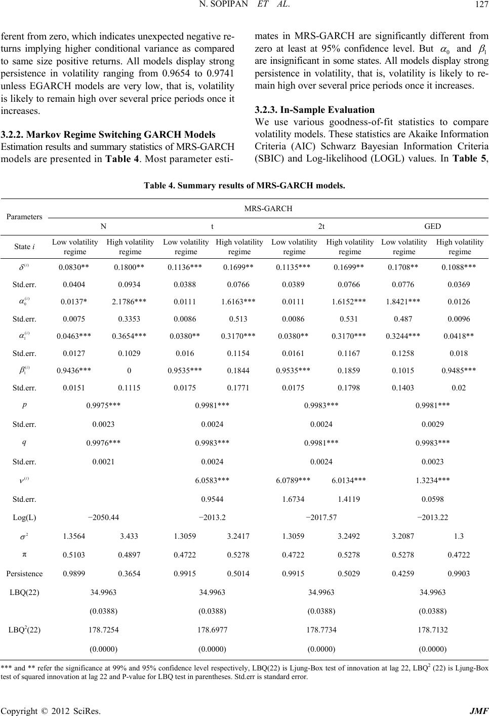

N. SOPIPAN ET AL. 127
ferent from zeh innexega
presented in Table 4. Most parameter esti-
MCHnifiiffe ro, whicdicates upected ntive re-
turns implying higher conditional variance as compared
o same size positive returns. All models display strong
zero at least at 95% confidence level. But 0
t
persistence in volatility ranging from 0.9654 to 0.9741
unless EGARCH models are very low, that is, volatility
is likely to remain high over several price periods once it
increases.
3.2.2. Markov Re gi me Switching GARCH Models
Estimation results and summary statistics of MRS-GARCH
models are
mates inRS-GAR are sigcantly drent from

and 1

are insignificant in some states. All models display strong
n
esian Information Criteria
s of
M
persistence in volatility, that is, volatility is likely to re-
main high over several price periods once it increases.
3.2.3. In-Sample Evaluation
We use various goodness-of-fit statistics to compare
volatility models. These statistics are Akaike Informatio
Criteria (AIC) Schwarz Bay
(SBIC) and Log-likelihood (LOGL) values. In Table 5,
MRS-GARCH models.
RS-GARCH
Table 4. Summary result
Parameters
N t 2t GED
State i Low volatility
regime
High volatility
regime
Low volatility
regime
High volatility
regi
Low volatility
me
High volatility
regime
Low volatility
regime
High volatility
regime me regi
()i

0.0830** 0.1800** 0.1136*** 0.1699** 0.1135*** 0.1699** 0.1708** *** 0.1088
Std.err.
()
0.0404 0.0934 0.0388 0.0766 0.0389 0.0766 0.0776 0.0369
0
i

0.0137* 2 1 1 1
Std.er. 0.0075
.1786***0.0111 .6163***0.0111 .6152***.8421*** 0.0126
r0.3353 0.0086 0.513 0.0086 0.531 0.487 0.0096
()i
1

0.04630.0380 0.31700.03800.3244 0.0418
Std.err. 0.0127
*** 0.3654*** ** *** ** 0.3170*** *** **
0.1029 0.016 0.1154 0.0161 0.1167 0.1258 0.018
()i
1

0.94360.95350.1844 0.0.1015 0.9485
Std.err. 0.0151
*** 0 *** 9535*** 0.1859 ***
0.1115 0.0175 0.1771 0.0175 0.1798 0.1403 0.02
p
0.9975*** 0.9981*** 0.9983*** 0.9981***
Std.err. 0.0023 0.0024 0.0024 0.0029
q 0.9976*** 0.9983*** 0.9981*** 0.9983***
Std.err. 0.0021 0.0024 0.0024 0.0023
()i

6.0789*** ***
1.4119
Log(L) −2050.44
6.0583*** 6.01341.3234***
Std.err. 0.9544 1.6734 0.0598
−2013.2 −2017.57 −2013.22
2

1.3564 3.433 1.3059 3.2417 3.2087 1.3
0.5103 0.4897 0.4722 0.4722 0.5278 0.5278
Persistence 0.9899 0.3654 0.9903
LBQ( 34.9963 34.9963 34.9963 34.9963
(0.0388) (0.0388) (0.0388) (0.0388)
LBQ2(22) 178.7254 178.6977 178.7734 178.7132
.0000) (0.0000)
1.3059 3.2492
π 0.5278 0.4722
0.9915 0.5014 0.9915 0.5029 0.4259
22)
(0(0.0000) (0.0000)
*** and ** refer the significance at(22) is Lox test of innovation at la LBQ2 (22) is Ljung-Box
test of squared inn
99% and 95% confidence level respectively, LBQjung-Bg 22,
ovation at lag 22 and P-value for LBQ test in parentheses. Std.err is standard error.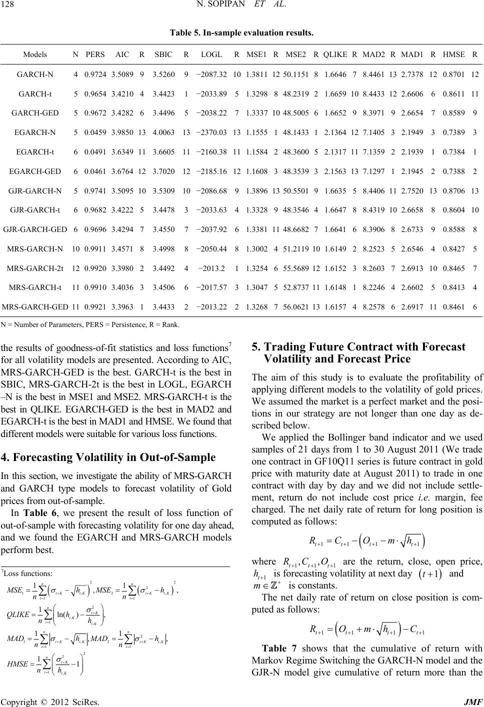

N. SOPIPAN ET AL. 128
Table 5. In-saaluatio.
s N PIC R SBIC R RMSE1RMSEIKER MAD2 R MAMSER
mple evn results
ModelERS ALOGL 2RQLD1 RH
GARCH-N 4 0.9724 089 9 3.5260 9 101.381112 50.114678.4461 13 2.7123.5 −2087.3251 81.66378 120.8701
GARCH-t 5 210 4 3.4423 1 51.3298848.2359 108.4433 12 2.6.861111
GARCH-GED 5 0.9672 282 6 3.4496 5 71.333710 48.50529 8.3971 9 2.69
EGARCH-t 6 0.0491 3.6349 11 3.662.1317 117.1359 2 2.1939 1 0.73841
EGAD 3 −
G
G-t
G
M
M2t
M
0.9654 3.4−2033.8919 21.66606 6 0
3.4 −2038.2205 61.66654 7 0.8589
EGARCH-N 5 0.0459 3.9850 13 4.0063 13−2370.03131.1555 148.14331 2.1364127.1405 3 2.1949 3 0.73893
05 11−2160.3811 1.15842 48.3600 5
RCH-GE6 0.0461 .676412 3.7020 122185.16121.1608 348.35393 2.1563137.1297 1 2.1945 2 0.73882
JR-GARCH-N5 0.9741 3.5095 10 3.5309 10−2086.6891.389613 50.550191.663558.4406 11 2.7520 130.870613
JR-GARCH6 0.9682 3.4222 5 3.4478 3 −2033.6341.33289 48.3546 41.664788.4319 10 2.6658 8 0.860410
JR-GARCH-GED 6 0.9696 3.4294 7 3.4550 7 −2037.9261.338111 48.668271.664168.3906 8 2.6733 9 0.85888
RS-GARCH-N 10 0.9911 3.4571 8 3.4998 8 −2050.4481.3002451.2119 101.6149 2 8.2523 5 2.6546 4 0.84275
RS-GARCH-12 0.9920 3.3980 2 3.4492 4 −2013.211.3254655.5689 121.615238.2603 7 2.6913 100.84657
MRS-GARCH-t 11 0.9910 3.4036 3 3.4506 6 −2017.5731.3047552.8737 111.6148 1 8.2246 4 2.6602 5 0.84134
RS-GARCH-GED 11 0.9921 3.3963 1 3.4433 2 −2013.2221.3268756.0621131.6157 4 8.2578 6 2.6917 110.84616
N e
s f
fd ,
MRS-GARCH-GED is the best. GARCH-t is the best in
S RL
–N MSE1RCH-
be the
f t
ctions.
nd Forecast Price
o
t
o-
tions in our strategy are not longer than one day as de-
We applied the Bollinger band indicator and we used
samples of 21 days from 1 to 30 August 2011 (We trade
one contract in GF10Q11 series is future contract in gold
ne
= Number of Paramters, PERS = Persistence, R = Rank.
the results of goodness-of-fit statistic and loss unctions7
or all volatility models are presented. Accoring to AIC
BIC, MRS-GACH-2t is the best in LOG, EGARCH
is the best in
st in QLIKE. EGA
and
RCH-GED i
MSE2.
s
MRS-GAt is the
andbest in MAD2
EGARCH-t is the best in MAD1 and HMSE. We ound tha
different models were suitable for various loss fun
4. Forecasting Volatility in Out-of-Sample
In this section, we investigate the ability of MRS-GARCH
and GARCH type models to forecast volatility of Gold
prices from out-of-sample.
In Table 6, we present the result of loss function of
out-of-sample with forecasting volatility for one day ahead,
and we found the EGARCH and MRS-GARCH models
perform best.
5. Trading Future Contract with Forecast
Volatility a
The aim
apply
of thi
g differ
s study is t
ent
evaluate t
o the v
he profitability of
tility oin models olaf gold prices.
We assumed the market is a perfect market and the psi
scribed below.
price with maturity date at August 2011) to trade in o
contract with day by day and we did not include settle-
ment, return do not include cost price i.e. margin, fee
charged. The net daily rate of return for long position is
computed as follows:


11 11tt tt
RC Omh
 
 
where 1 ,,
tt
RCO
1t1


are the return, close, open price,
1t
h

is forecasting volatility at next day

1t and
m

 is constants.
The net daily rate of return on close position is com-
puted as follows:


11 11tt tt
ROmhC


 
Table 7 shows that the cumulative of return with
Markov Regime Switching the GARCH-N model and the
JR-N model give cumulative of return more than the G
7Loss functions:


22
2
1,2
11
2
,
1,
2
1,2
11
2
2
1,
11
,,
1ln( ),
11
,,
11
nn
t KtKtKtK
tt
n
tK
tK
ttK
nn
t KtKt KtK
tt
n
tK
ttK
MSEh MSEh
nn
QLIKE h
nh
MADh MADh
nn
HMSE nh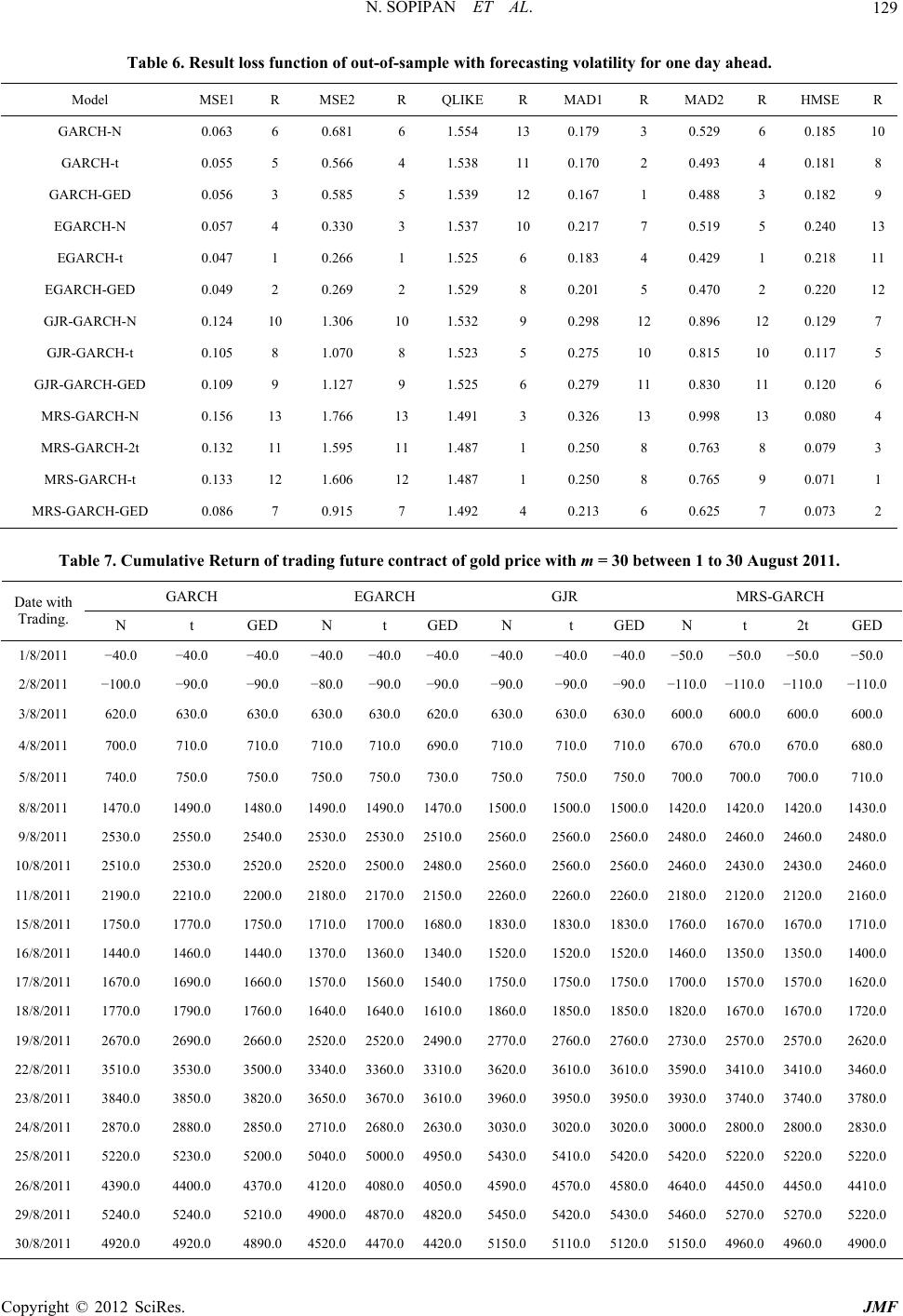


















 









,
,

N. SOPIPAN ET AL. 129
Table 6. Result loss function of out-of-sampl
Model MSE1 R MSE2 R
orecasting volatility for one day ahead. e with f
QLIKE R MAD1 R MAD2 R HMSE R
GARCH-N 0.063 6 0.681 6 1.53 0.529 6 0.185 1054 13 0.179
GARCH-t 0.055 5 0.566 4
GARCH-GED
1.538 11 0.170 2 0.493 4 0.181 8
0.056 3 0.585 5 1.539
EGARCH-N 0.057 4 0 3 1.5
EGARCH-t 1.5
EGARCH-GE0.220 12
GJR-N
G
GJRED
M
Mt
M
M
12 0.167 1 0.488 3 0.182 9
37 10 0.217 7 0.519 5 0.240 13
25 6 0.183 4 0429 1 0.218 11
0.33
0.047 1 0.266 1 .
D 0.049 2 0.269 2 1.529 8 0.201 5 0.470 2
-GARCH0.124 10 1.306 10 1.532 9 0.298 12 0.896 12 0.129 7
JR-GARCH-t 0.105 8 1.070 8 1.523 5 0.275 10 0.815 10 0.117 5
-GARCH-G0.109 9 1.127 9 1.525 6 0.279 11 0.830 11 0.120 6
RS-GARCH-N0.156 13 1.766 13 1.491 3 0.326 13 0.998 13 0.080 4
RS-GARCH-20.132 11 1.595 11 1.487 1 0.250 8 0.763 8 0.079 3
RS-GARCH-t 0.133 12 1.606 12 1.487 1 0.250 8 0.765 9 0.071 1
RS-GARCH-GED0.086 7 0.915 7 1.492 4 0.213 6 0.625 7 0.073 2
ulativrn adiure cracld price wi 30 een0 Aust
GARCH EGARCH GJR MRS-GARCH
Table 7. Cume Retuof trng futontt of goth m =betw 1 to 3ug 2011.
Date with
Tr GED t GEDN GEDNt 2t GED ading. N t N t
1/8/ −40. −40 −−40. −4−40. − −40. −5−50. −5−50.2011 −40.0 0 .0 40.0 00.00 40.000.0 0 0.00
2/8/ −90. −90 −−90. −9−90. − −90. −11110. −11 −11
3/8/630.630.6630. 62630.63630. 60600. 60600
4/710.710.7710. 69710.71710. 67670. 67680
5/8/20710.0
8/8/2011 1470.0 1490.0 1480.0 1490.0 1490.01470.0 1500.0 1500.01500.01420.0 1420.0 1420.0 1430.0
2530.0 2540.0 2530.0 2510.0 2560.0 2502560.02480.0 242480.0
10/8/2011 250 2530.0 250 2502250 2560.02240 2430.0 240 2
11/21222221 222
15/171717 11
16/14141413 11113131
2011 −100.0 0 .0 80.0 00.00 90.000.0 −0 0.00.0
2011 620.0 0 0 30.0 0 0.00 0.000.0 0 0.0.0
8/2011 700.0 0 0 10.0 00.00 0.00 0.0 0 0.0.0
11 740.0 750.0 750.0 750.0 750.0730.0750.0 750.0750.0700.0 700.0 700.0
9/8/2011 2550.0 2530.060.60.0 2460.0
10.20.0 2520.00.480.060.560.060.30.460.0
8/2011 90.0 10.0 00.0 2180.0 70.0150.0 2260.0 2260.0260.02180.0 2120.0 2120.0160.0
8/2011 1750.0 70.0 50.0 1710.0 00.0680.0 1830.0 1830.0 830.01760.0 1670.0 1670.0 1710.0
8/2011 40.0 60.0 40.0 1370.0 60.0340.0520.0 1520.0 520.01460.0 50.0 50.0400.0
17/8/2011 1670.0 1690.0 1660.0 1570.0 1560.01540.0 1750.0 1750.01750.01700.0 1570.0 1570.0 1620.0
18/8/2011 1770.0 1790.0 1760.0 1640.0 1640.01610.0 1860.0 1850.01850.01820.0 1670.0 1670.0 1720.0
19/8/2011 2670.0 2690.0 2660.0 2520.0 2520.02490.0 2770.0 2760.02760.02730.0 2570.0 2570.0 2620.0
22/8/2011 3510.0 3530.0 3500.0 3340.0 3360.03310.0 3620.0 3610.03610.03590.0 3410.0 3410.0 3460.0
23/8/2011 3840.0 3850.0 3820.0 3650.0 3670.03610.0 3960.0 3950.03950.03930.0 3740.0 3740.0 3780.0
24/8/2011 2870.0 2880.0 2850.0 2710.0 2680.02630.0 3030.0 3020.03020.03000.0 2800.0 2800.0 2830.0
25/8/2011 5220.0 5230.0 5200.0 5040.0 5000.04950.0 5430.0 5410.05420.05420.0 5220.0 5220.0 5220.0
26/8/2011 4390.0 4400.0 4370.0 4120.0 4080.04050.0 4590.0 4570.04580.04640.0 4450.0 4450.0 4410.0
29/8/2011 5240.0 5240.0 5210.0 4900.0 4870.04820.0 5450.0 5420.05430.05460.0 5270.0 5270.0 5220.0
30/8/2011 4920.0 4920.0 4890.0 4520.0 4470.04420.0 5150.0 5110.05120.05150.0 4960.0 4960.0 4900.0

N. SOPIPAN ET AL. 130
ols we=
6. Conclusions
Inerrelat gin
Markov RegimRSd
emlloatihfy
nor unede e
n e opapo he
MRSH ms are aimprovemente GARCH
s ncR1)R,1
modeling and fore-
casting gold price closed price volatility. We compare
models with GARCH (1,1), EGARCH
.g. EGARCH, GJR. In addition, the per-
fo SCdned
fur ldps
7.ogt
Th y
refu G
E C
[1] e“s
ther mode when use m 30.
this pap, we fo
e Switch
cast vo
ing GARC
ility of
H (M
old pr
-GARC
ces usi
H) mo
g
-
ls. These odels aw vollity to ave diferent d-
amics accding toobserv regimvariabls.
The maipurposf this er is tfind out whetr
-GARC
pe model
odel
which i
n
lude GA
on th
, EGAtyCH (1,CH (1)
and GJR-GARCH (1,1) in terms of
MRS-GARCH (1,1)
(1,1), GJR-GARCH (1,1) models. All models are esti-
mated under three distributional assumptions which are
Nor- mal, Student-t and GED. Moreover, Student-t distribu-
tion which takes different degrees of freedom in each re-
gime is considered for MRS-GARCH models.
We first analyze in-sample performance of various
volatility models to determine the best form of the vola-
tility model over the period 4/01/2007 through 30/08/2011.
As expected, volatility is not constant over time and ex-
hibits volatility clustering showing large changes in the
price of an asset often followed by large changes, and small
changes often followed by small changes.
Descriptive statistics of return series are represented
by returns with fatter tails. The Augmented Dickey-
Fuller test indicates gold price log returns are stationary.
Serial correlation in the gold price confirms it is non-
stationary but serial log returns of gold price are station-
ary. Serial correlation in the squared returns suggests condi-
tional heteroskedasticity. This empirical part adopts
GARCH type and MRS-GARCH models to estimate the
volatility of the gold price. In order to account for fat
tailed features of financial returns, we consider three dif-
ferent distributions for the innovations. Almost all pa-
rameter estimates in GARCH type models are highly sig-
nificant at 1%. Most parameter estimates in MRS-GARCH
are significantly different from zero at least at 95% confi-
dence level. However, the results of goodness-of-fit statis-
tics and loss functions for all volatility models show dif-
ferent results.
The trading details we have used describe forecasts of
closed price of gold price between 1/08/2011-30/08/2011
and trading in gold future contract (GF10Q11). We found
the cumulative returns with the Markov Regime Switch-
ing GARCH-N (MRS-GARCH-N) model and the GJR-N
model give us higher cumulative returns than the other
models when we use m = 30.
For further study, three or four volatility regimes set-
ting can be considered rather than two-volatility regimes.
Also, using Markov Regime Switching with other vola-
tility models e
rmance of MR -GARH moels ca be hged in
ture foong an short osition.
Acknwledemens
is research is (partially) supported b the Thailand
search nd BR.
REFRENES
A. Mhmet, Analysiof Turkish Financial Market with
Markov Regime Switching Volatility Models,” The Mid-
dle East Technical University, Ankara, 2008.
[2] R. Engle, “Autoregressive Conditional Heteroscedasticity
with Estimates of the Variance of United Kingdom Infla-
tion,” Econometrica, Vol. 50, No. 4, 1982, pp. 987-1008.
doi:10.2307/1912773
[3] T. Bollerslev, “Generalized Autoregressive Conditional
Heteroscedasticity,” Journal of Econometrics, Vol. 31, No. 3,
1986, pp. 307-327. doi:10.1016/0304-4076(86)90063-1
[4] D. B. Nelson, “Conditional Heteroskedasticity in Asset
Returns: A New Approach,” Econometrica, Vol. 59, No.
2, 1991, pp. 347-370. doi:10.2307/2938260
[5] L. R. Glosten, R. Jagannathan and D. Runkle, “On the
Relation between the Expected Value and the Nominal
Excess Return on Financials,” Journal of Finance, Vol.
801. doi:10.2307/232906748, No. 5, 1993, pp. 1779-1
ics, Vol. 64, No. 1-2, 1994, pp. 307-333.
doi:10.1016/0304-4076(94)90067-1
[6] J. D. Haminton and R. Susmel, “Autoregressive Condi-
tional Heteroskedasticity and Change in Regime,” Jour-
nal of Econometr
[7] Z. F. Guo anransition GARCH
Model with Asases,” Proceedings
CE2011_pp
JAM/issues_v41/issue_4/IJAM_41
Uni-
ity of Dublin,
d L. Cao, “A Smooth T
ymmetric Transition Ph
of International Conference of Financial Engineering, Lon-
don, 6-8 July 2011.
http://www.iaeng.org/publication/WCE 2011/W
439-441.pdf
[8] Z. F. Guo and L. Cao, “An Asymmetric Smooth Transi-
tion GARCH Model,” IAENG Journals, 2011.
http://www.iaeng.org/I
_4_10.pdf
[9] J. Marcucci, “Forecasting Financial Market Volatility with
Regime-Switching GARCH Model,” Working Paper,
versity of California, San Diego, 2005.
[10] T. Edel and M. Brian, “APGARCH Investigation of the
Main Influences on the Gold Price,” Univers
Dublin, 2005.
[11] S. Gray, “Modeling the Conditional Distribution of Inte-
rest Rates as a Regime-Switching Process,” Journal of Fi-
nancial Economics, Vol. 42, No. 1, 1996, pp. 27-62.
doi:10.1016/0304-405X(96)00875-6
[12] F. Klaanssen, “Improving GARCH Volatility Forecasts
with Regime-Switching GARCH,” Empirical Economics,
Vol. 27, No. 2, 2002, pp. 363-394.
doi:10.1007/s001810100100
[13] C. J. Kimand and C. R. Nelson, “State-Space Models with
Regime Switching: Classical and Gibbs-Sampling Approa-

N. SOPIPAN ET AL. 131
ches with Applications
[14] J. D. Hamilton, “A New Approach to the Economic Ana-
lysis of Nons
,” MIT Press, Cambridge, 1999.
tationary Time Series and the Business Cy-
cle,” Econometrica, Vol. 57, No. 2, 1989, pp. 357-384.
doi:10.2307/1912559
[15] J. D. Hamilton, “Analysis of Time Series Subject to Change
in Regime,” Journal of Econometrics
pp. 39-70.
, Vol. 45, No. 1-2, 1990,
76(90)90093-9doi:10.1016/0304-40
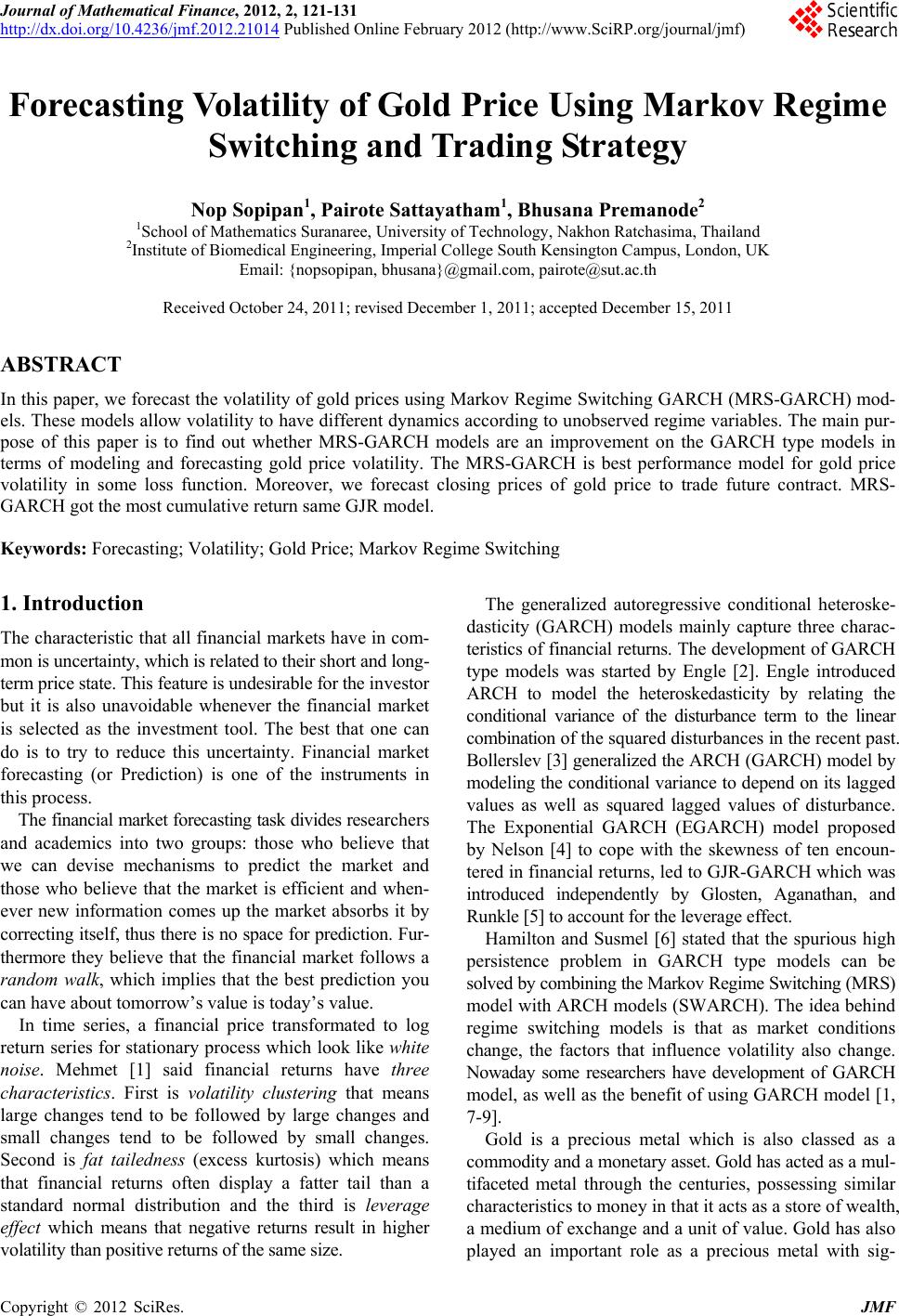