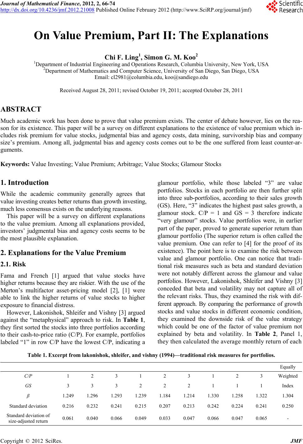
Journal of Mathematical Finance, 2012, 2, 66-74
http://dx.doi.org/10.4236/jmf.2012.21008 Published Online February 2012 (http://www.SciRP.org/journal/jmf)
On Value Premium, Part II: The Explanations
Chi F. Ling1, Simon G. M. Koo2
1Department of Industrial Engineering and Operations Research, Columbia University, New York, USA
2Department of Mathematics and Computer Science, University of San Diego, San Diego, USA
Received August 28, 2011; revised October 19, 2011; accepted October 28, 2011
ABSTRACT
Much academic work has been done to prove that value premium exists. The center of debate however, lies on the rea-
son for its existence. This paper will be a survey on different explanations to the existence of value premium which in-
cludes risk premium for value stocks, judgmental bias and agency costs, data mining, survivorship bias and company
size’s premium. Among all, judgmental bias and agency costs comes out to be the one suffered from least counter-ar-
guments.
Keywords: Value Investing; Value Premium; Arbitrage; Value Stocks; Glamour Stocks
1. Introduction
While the academic community generally agrees that
value investing creates better returns than growth investing,
much less consensus exists on the underlying reasons.
This paper will be a survey on different explanations
to the value premium. Among all explanations provided,
investors’ judgmental bias and agency costs seems to be
the most plausible explanation.
2. Explanations for the Value Premium
2.1. Risk
Fama and French [1] argued that value stocks have
higher returns because they are riskier. With the use of the
Merton’s multifactor asset-pricing model [2], [1] were
able to link the higher returns of value stocks to higher
exposure to financial distress.
However, Lakonishok, Shleifer and Vishny [3] argued
against the “metaphysical” approach to risk. In Table 1,
they first sorted the stocks into three portfolios according
to their cash-to-price ratio (C/P). For example, portfolios
labeled “1” in row C/P have the lowest C/P, indicating a
glamour portfolio, while those labeled “3” are value
portfolios. Stocks in each portfolio are then further split
into three sub-portfolios, according to their sales growth
(GS). Here, “3” indicates the highest past sales growth, a
glamour stock. C/P = 1 and GS = 3 therefore indicate
“very glamour” stocks. Value portfolios were, in earlier
part of the paper, proved to generate superior return than
glamour portfolio (The superior return is often called the
value premium. One can refer to [4] for the proof of its
existence). The point here is to examine the risk between
value and glamour portfolio. One can notice that tradi-
tional risk measures such as beta and standard deviation
were not notably different across the glamour and value
portfolios. However, Lakonishok, Shleifer and Vishny [3]
conceded that beta and volatility may not capture all of
the relevant risks. Thus, they examined the risk with dif-
ferent approach. By comparing the performance of growth
stocks and value stocks in different economic condition,
they examined the downside risk of the value strategy
which could be one of the factor of value premium not
explained by beta and volatility. In Table 2, Panel 1,
they then calculated the average monthly return of each
Table 1. Excerpt from lakonishok, shleifer, and vishny (1994)—traditional risk measures for portfolios.
Equally
C/P 1 2 3 1 2 3 1 2 3 Weighted
GS 3 3 3 2 2 2 1 1 1 Index
β 1.249 1.296 1.293 1.239 1.184 1.214 1.330 1.258 1.322 1.304
Standard deviation 0.216 0.232 0.241 0.215 0.207 0.213 0.242 0.224 0.241 0.250
Standard deviation of
size-adjusted return 0.061 0.040 0.066 0.049 0.033 0.047 0.066 0.047 0.065 -
C
opyright © 2012 SciRes. JMF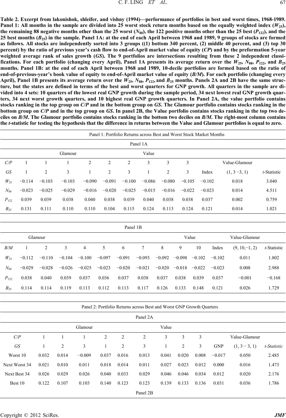

C. F. LING ET AL. 67
Table 2. Excerpt from lakonishok, shleifer, and vishny (1994)—performance of portfolios in best and worst times, 1968-1989.
Panel 1: All months in the sample are divided into 25 worst stock return months based on the equally weighted index (W25),
the remaining 88 negative months other than the 25 worst (N88), the 122 positive months other than the 25 best (P122), and the
25 best months (B25) in the sample. Panel 1A: at the end of each April between 1968 and 1989, 9 groups of stocks are formed
as follows. All stocks are independently sorted into 3 groups ((1) bottom 340 percent, (2) middle 40 percent, and (3) top 30
percent) by the ratio of previous year’s cash flow to end-of-April market value of equity (CP) and by the preformation 5-year
weighted average rank of sales growth (GS). The 9 portfolios are intersections resulting from these 2 independent classi-
fications. For each portfolio (changing every April), Panel 1A presents its average return over the W25, N88, P122, and B25
months. Panel 1B: at the end of each April between 1968 and 1989, 10-decile portfolios are formed based on the ratio of
end-of-previous-year’s book value of equity to end-of-April market value of equity (B/M). For each portfolio (changing every
April), Panel 1B presents its average return over the W25, N88, P122, and B25 months. Panels 2A and 2B have the same struc-
ture, but the states are defined in terms of the best and worst quarters for GNP growth. All quarters in the sample are di-
vided into 4 sets: 10 quarters of the lowest real GNP growth during the sample period, 34 next lowest real GNP growth quar-
ters, 34 next worst growth quarters, and 10 highest real GNP growth quarters. In Panel 2A, the value portfolio contains
stocks ranking in the top group on C/P and in the bottom group on GS. The Glamour portfolio contains stocks ranking in the
bottom group on C/P and in the top group on GS. In panel 2B, the Value portfolio contains stocks ranking in the top two de-
ciles on B/M. The Glamour portfolio contains stocks ranking in the bottom two deciles on B/M. The right-most column contains
the t-statistic for testing the hypothesis that the difference in returns between the Value and Glamour portfolios is equal to zero.
Panel 1: Portfolio Returns across Best and Worst Stock Market Months
Panel 1A
Glamour Value
C/P 1 1 1 2 2 2 3 3 3 Value-Glamour
GS 1 2 3 1 2 3 1 2 3 Index(1, 3 −3, 1) t-Statistic
W25 −0.114 −0.103 −0.103 −0.090 −0.091 −0.100 −0.086 −0.080 −0.105 −0.1020.018 3.040
N88 −0.023 −0.025 −0.029 −0.016 −0.020 −0.025 −0.015 −0.016 −0.022 −0.0230.014 4.511
P122 0.039 0.039 0.038 0.040 0.0380.0390.0400.0380.0380.0370.002 0.759
B25 0.131 0.111 0.110 0.110 0.1040.1150.1240.1130.1240.1210.014 1.021
Panel 1B
Glamour Value Value-Glamour
B/M 1 2 3 4 5 6 7 8 9 10 Index (9, 10,−1, 2) t-Statistic
W25 −0.112 −0.110 −0.104 −0.100 −0.097 −0.091 −0.093 −0.092 −0.098 −0.102 −0.102 0.011 1.802
N88 −0.029 −0.028 −0.026 −0.025 −0.023 −0.020 −0.021 −0.020 −0.018−0.022−0.023 0.008 2.988
P122 0.038 0.040 0.0390.037 0.036 0.037 0.038 0.0370.0380.0390.037 −0.001 −0.168
B25 0.114 0.114 0.1190.113 0.112 0.113 0.117 0.1260.1330.1480.121 0.026 1.729
Panel 2: Portfolio Returns across Best and Worst GNP Growth Quarters
Panel 2A
Glamour Value
C/P 1 1 1 2 2 2 3 3 3 Value-Glamour
GS 1 2 3 1 2 3 1 2 3 GNP (1, 3 − 3, 1) t-Statistic
Worst 10 0.032 0.014 −0.009 0.037 0.0160.013 0.0410.0200.008−0.017 0.050 2.485
Next Worst 34 0.021 0.010 0.011 0.018 0.0140.011 0.0270.0230.0120.000 0.016 1.473
Next Best 34 0.026 0.029 0.026 0.040 0.0330.029 0.0460.0460.0340.012 0.020 2.176
Best 10 0.122 0.107 0.103 0.140 0.1230.123 0.1390.1330.1360.031 0.036 1.786
Panel 2B

C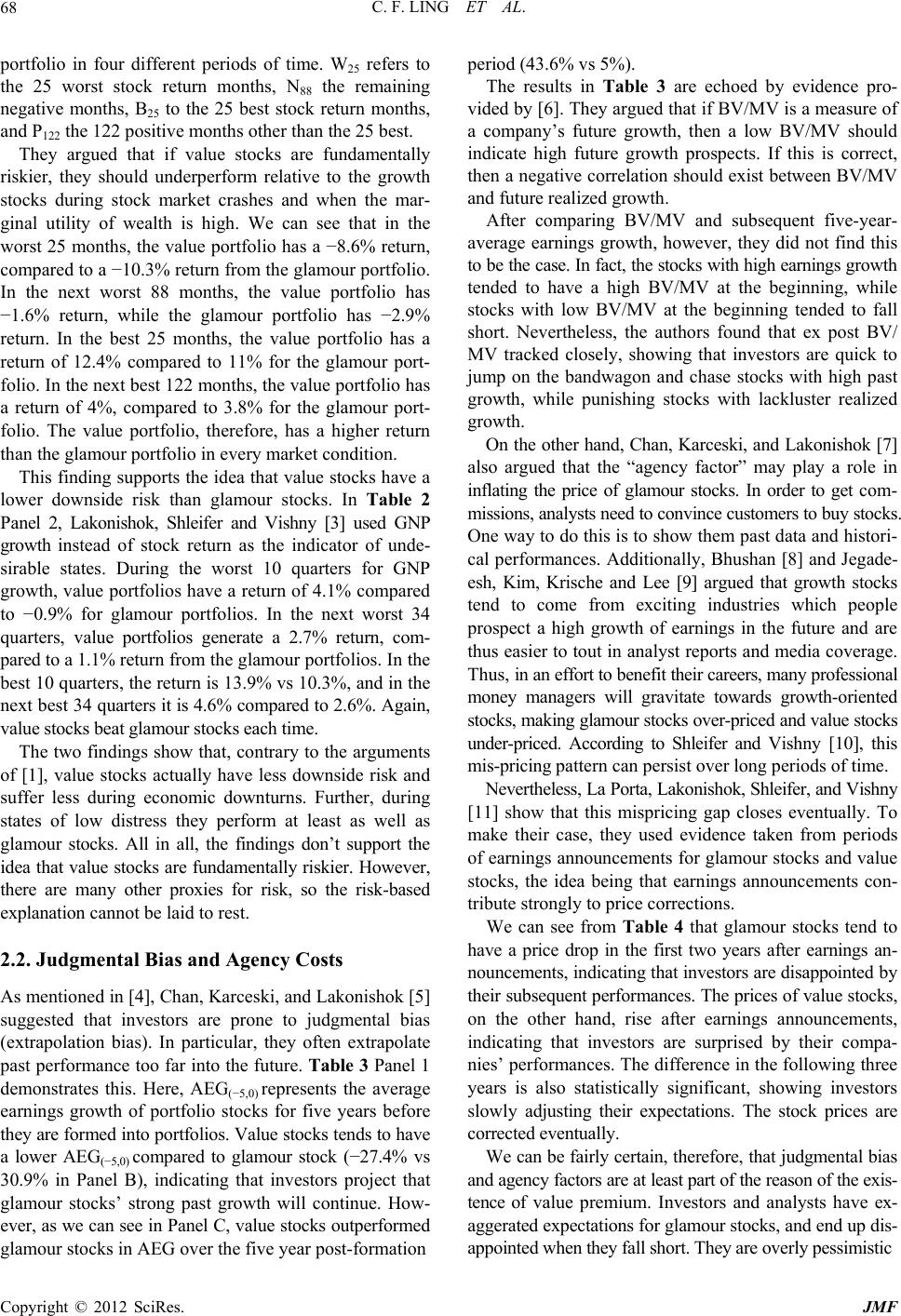. F. LING ET AL. 68
portfolio in four different periods of time. W25 refers to
the 25 worst stock return months, N88 the remaining
negative months, B25 to the 25 best stock return months,
and P122 the 122 positive months other than the 25 best.
They argued that if value stocks are fundamentally
riskier, they should underperform relative to the growth
stocks during stock market crashes and when the mar-
ginal utility of wealth is high. We can see that in the
worst 25 months, the value portfolio has a −8.6% return,
compared to a −10.3% return from the glamour portfolio.
In the next worst 88 months, the value portfolio has
−1.6% return, while the glamour portfolio has −2.9%
return. In the best 25 months, the value portfolio has a
return of 12.4% compared to 11% for the glamour port-
folio. In the next best 122 months, the value portfolio has
a return of 4%, compared to 3.8% for the glamour port-
folio. The value portfolio, therefore, has a higher return
than the glamour portfolio in every market condition.
This finding supports the idea that value stocks have a
lower downside risk than glamour stocks. In Table 2
Panel 2, Lakonishok, Shleifer and Vishny [3] used GNP
growth instead of stock return as the indicator of unde-
sirable states. During the worst 10 quarters for GNP
growth, value portfolios have a return of 4.1% compared
to −0.9% for glamour portfolios. In the next worst 34
quarters, value portfolios generate a 2.7% return, com-
pared to a 1.1% return from the glamour portfolios. In the
best 10 quarters, the return is 13.9% vs 10.3%, and in the
next best 34 quarters it is 4.6% compared to 2.6%. Again,
value stocks beat glamour stocks each time.
The two findings show that, contrary to the arguments
of [1], value stocks actually have less downside risk and
suffer less during economic downturns. Further, during
states of low distress they perform at least as well as
glamour stocks. All in all, the findings don’t support the
idea that value stocks are fundamentally riskier. However,
there are many other proxies for risk, so the risk-based
explanation cannot be laid to rest.
2.2. Judgmental Bias and Agency Costs
As mentioned in [4], Chan, Karceski, and Lakonishok [5]
suggested that investors are prone to judgmental bias
(extrapolation bias). In particular, they often extrapolate
past performance too far into the future. Table 3 Panel 1
demonstrates this. Here, AEG(−5,0) represents the average
earnings growth of portfolio stocks for five years before
they are formed into portfolios. Value stocks tends to have
a lower AEG(−5,0) compared to glamour stock (−27.4% vs
30.9% in Panel B), indicating that investors project that
glamour stocks’ strong past growth will continue. How-
ever, as we can see in Panel C, value stocks outperformed
glamour stocks in AEG over the five year post-formation
period (43.6% vs 5%).
The results in Table 3 are echoed by evidence pro-
vided by [6]. They argued that if BV/MV is a measure of
a company’s future growth, then a low BV/MV should
indicate high future growth prospects. If this is correct,
then a negative correlation should exist between BV/MV
and future realized growth.
After comparing BV/MV and subsequent five-year-
average earnings growth, however, they did not find this
to be the case. In fact, the stocks with high earnings growth
tended to have a high BV/MV at the beginning, while
stocks with low BV/MV at the beginning tended to fall
short. Nevertheless, the authors found that ex post BV/
MV tracked closely, showing that investors are quick to
jump on the bandwagon and chase stocks with high past
growth, while punishing stocks with lackluster realized
growth.
On the other hand, Chan, Karceski, and Lakonishok [7]
also argued that the “agency factor” may play a role in
inflating the price of glamour stocks. In order to get com-
missions, analysts need to convince customers to buy stocks.
One way to do this is to show them past data and histori-
cal performances. Additionally, Bhushan [8] and Jegade-
esh, Kim, Krische and Lee [9] argued that growth stocks
tend to come from exciting industries which people
prospect a high growth of earnings in the future and are
thus easier to tout in analyst reports and media coverage.
Thus, in an effort to benefit their careers, many professional
money managers will gravitate towards growth-oriented
stocks, making glamour stocks over-priced and value stocks
under-priced. According to Shleifer and Vishny [10], this
mis-pricing pattern can persist over long periods of time.
Nevertheless, La Porta, Lakonishok, Shleifer, and Vishny
[11] show that this mispricing gap closes eventually. To
make their case, they used evidence taken from periods
of earnings announcements for glamour stocks and value
stocks, the idea being that earnings announcements con-
tribute strongly to price corrections.
We can see from Table 4 that glamour stocks tend to
have a price drop in the first two years after earnings an-
nouncements, indicating that investors are disappointed by
their subsequent performances. The prices of value stocks,
on the other hand, rise after earnings announcements,
indicating that investors are surprised by their compa-
nies’ performances. The difference in the following three
years is also statistically significant, showing investors
slowly adjusting their expectations. The stock prices are
corrected eventually.
We can be fairly certain, therefore, that judgmental bias
and agency factors are at least part of the reason of the exis-
tence of value premium. Investors and analysts have ex-
aggerated expectations for glamour stocks, and end up dis-
appointed when they fall short. They are overly pessimistic

C. F. LING ET AL. 69
Table 3. Excerpt from Lakonishok, Shleifer, and Vishny (1994)—Fundamental variables, past performance, and future
performance of glamour and value stocks, 1968-1989. Panel 1: at the end of each April between 1968 and 1989, 10-decile
portfolios are formed based on the ratio of end-of-previous-year’s book value of equity to end-of-April market value of equity.
Numbers are presented for the first (lowest B/M) and tenth (highest B/M) deciles. These portfolios are denoted Glamour and
Value, respectively. Panel 2: at the end of each April between 1968 and 1989, 9 groups of stocks are formed. The stocks are
independently sorted in ascending order into 3 groups ((1) bottom 30 percent, (2) middle 40 percent, (3) top 30 percent) based
on C/P, the ratio of cash flow to market value of equity, and GS, the preformation 5-year weighted average sales growth rank.
Numbers are presented for (C/P1, GS3), the bottom 30 percent by C/P and the top 30 percent by GS, and for (C/P3, GS1) the
top 30 percent by C/P and the bottom 30 percent by GS. These portfolios are denoted Glamour and Value, respectively. All
numbers in the table are averages over all formation periods. E/P, C/P, S/P, D/P, B/M, and SIZE, defined below, use the
end-of-April market value of equity and preformation year accounting numbers. E/P is the ratio of earnings to market value
of equity. S/P is the ratio of sales to market value of equity. D/P is the ratio of dividends to market value of equity. B/M is the
ratio of book value to market value of equity. SIZE is the total dollar value of equity (in millions). AEG(i, j) is the geometric
average growth rate of earnings for the portfolio from year i to year j. ACG(i, j) and ASG(i, j) are defined analogously for cash
flow and sales, respectively. RETURN(−3, 0) is the cumulative stock return on the portfolio over the 3 years prior to formation.
Panel 1 Panel 2
Glamour Value Glamour Value
B/M1 B/M10 C/P1, GS3 C/P3, GS1
Panel A: Fundamental Variables
E/P 0.029 0.004 0.054 0.114
C/P 0.059 0.172 0.080 0.279
S/P 0.993 6.849 1.115 5.279
D/P 0.012 0.032 0.014 0.039
B/M 0.225 1.998 0.385 1.414
SIZE 663 120 681 390
Panel B: Past Performance—Growth Rates and Past Returns
AEG(−5, 0) 0.309 −0.274 0.142 0.082
ACG(−5, 0) 0.217 −0.013 0.210 0.078
ASG(−5, 0) 0.091 0.030 0.112 0.013
RETURN(−5, 0) 1.455 −0.119 1.390 0.225
Panel C: Future Performance
AEG(0, 5) 0.050 0.436 0.089 0.086
ACG(0, 5) 0.127 0.070 0.112 0.052
ASG(0, 5) 0.062 0.020 0.100 0.037
AEG(2, 5) 0.070 0.215 0.084 0.147
ACG(2, 5) 0.086 0.111 0.095 0.088
ASG(2, 5) 0.059 0.023 0.082 0.038
about value stocks, and end up being surprised by their
strong performances.
2.3. Data-Mining
Lo and MacKinlay [12] argued that the findings of value
premium were the result of data-mining; that is, attempt-
ing to find a pattern that lacks prediction power. Chan,
Hamao, and Lakonishok [13] addressed this concern by
studying the Japanese stock market. The result is shown
in Table 5. Sorted by BV/MV (Panel C), the value port-
folio (4) has an average monthly return of 2.43%, com-
pared to 1.13% of the glamour portfolio (1). Sorted by
CF/P (Panel D), the value portfolio has an average
monthly return of 2.22%, whereas the glamour portfo-
lio’s is 1.43%. Note that thandard deviation of the e st

C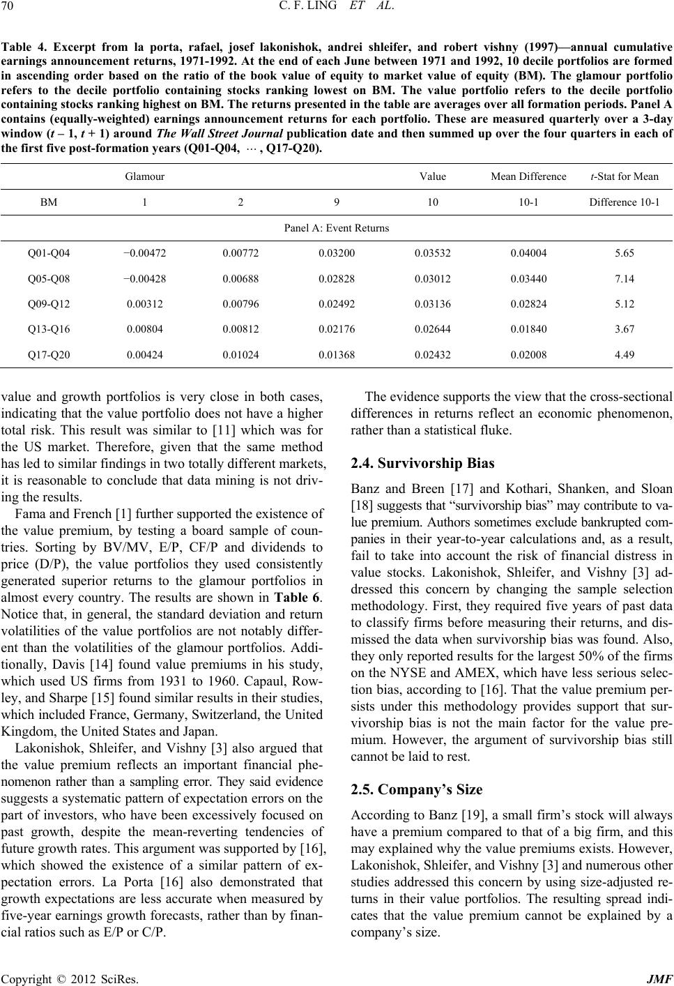. F. LING ET AL. 70
Table 4. Excerpt from la porta, rafael, josef lakonishok, andrei shleifer, and robert vishny (1997)—annual cumulative
earnings announcement returns, 1971-1992. At the end of each June between 1971 and 1992, 10 decile portfolios are formed
in ascending order based on the ratio of the book value of equity to market value of equity (BM). The glamour portfolio
refers to the decile portfolio containing stocks ranking lowest on BM. The value portfolio refers to the decile portfolio
containing stocks ranking highest on BM. The returns presented in the table are averages over all formation periods. Panel A
contains (equally-weighted) earnings announcement returns for each portfolio. These are measured quarterly over a 3-day
window (t – 1, t + 1) around The Wall Street Journal publication date and then summed up over the four quarters in each of
the first five post-formation years (Q01-Q04, , Q17-Q20). 
Glamour Value Mean Difference t-Stat for Mean
BM 1 2 9 10 10-1 Difference 10-1
Panel A: Event Returns
Q01-Q04 −0.00472 0.00772 0.03200 0.03532 0.04004 5.65
Q05-Q08 −0.00428 0.00688 0.02828 0.03012 0.03440 7.14
Q09-Q12 0.00312 0.00796 0.02492 0.03136 0.02824 5.12
Q13-Q16 0.00804 0.00812 0.02176 0.02644 0.01840 3.67
Q17-Q20 0.00424 0.01024 0.01368 0.02432 0.02008 4.49
value and growth portfolios is very close in both cases,
indicating that the value portfolio does not have a higher
total risk. This result was similar to [11] which was for
the US market. Therefore, given that the same method
has led to similar findings in two totally different markets,
it is reasonable to conclude that data mining is not driv-
ing the results.
Fama and French [1] further supported the existence of
the value premium, by testing a board sample of coun-
tries. Sorting by BV/MV, E/P, CF/P and dividends to
price (D/P), the value portfolios they used consistently
generated superior returns to the glamour portfolios in
almost every country. The results are shown in Table 6.
Notice that, in general, the standard deviation and return
volatilities of the value portfolios are not notably differ-
ent than the volatilities of the glamour portfolios. Addi-
tionally, Davis [14] found value premiums in his study,
which used US firms from 1931 to 1960. Capaul, Row-
ley, and Sharpe [15] found similar results in their studies,
which included France, Germany, Switzerland, the United
Kingdom, the United States and Japan.
Lakonishok, Shleifer, and Vishny [3] also argued that
the value premium reflects an important financial phe-
nomenon rather than a sampling error. They said evidence
suggests a systematic pattern of expectation errors on the
part of investors, who have been excessively focused on
past growth, despite the mean-reverting tendencies of
future growth rates. This argument was supported by [16],
which showed the existence of a similar pattern of ex-
pectation errors. La Porta [16] also demonstrated that
growth expectations are less accurate when measured by
five-year earnings growth forecasts, rather than by finan-
cial ratios such as E/P or C/P.
The evidence supports the view that the cross-sectional
differences in returns reflect an economic phenomenon,
rather than a statistical fluke.
2.4. Survivorship Bias
Banz and Breen [17] and Kothari, Shanken, and Sloan
[18] suggests that “survivorship bias” may contribute to va-
lue premium. Authors sometimes exclude bankrupted com-
panies in their year-to-year calculations and, as a result,
fail to take into account the risk of financial distress in
value stocks. Lakonishok, Shleifer, and Vishny [3] ad-
dressed this concern by changing the sample selection
methodology. First, they required five years of past data
to classify firms before measuring their returns, and dis-
missed the data when survivorship bias was found. Also,
they only reported results for the largest 50% of the firms
on the NYSE and AMEX, which have less serious selec-
tion bias, according to [16]. That the value premium per-
sists under this methodology provides support that sur-
vivorship bias is not the main factor for the value pre-
mium. However, the argument of survivorship bias still
cannot be laid to rest.
2.5. Company’s Size
According to Banz [19], a small firm’s stock will always
have a premium compared to that of a big firm, and this
may explained why the value premiums exists. However,
Lakonishok, Shleifer, and Vishny [3] and numerous other
studies addressed this concern by using size-adjusted re-
turns in their value portfolios. The resulting spread indi-
cates that the value premium cannot be explained by a
company’s size.

C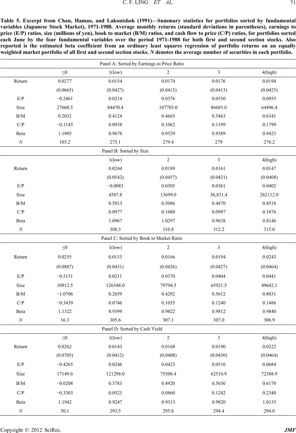. F. LING ET AL. 71
Table 5. Excerpt from Chan, Hamao, and Lakonishok (1991)—Summary statistics for portfolios sorted by fundamental
variables (Japanese Stock Market), 1971-1988. Average monthly returns (standard deviations in parentheses), earnings to
price (E/P) ratios, size (millions of yen), book to market (B/M) ratios, and cash flow to price (C/P) ratios, for portfolios sorted
each June by the four fundamental variables over the period 1971-1988 for both first and second section stocks. Also
reported is the estimated beta coefficient from an ordinary least squares regression of portfolio returns on an equally
weighted market portfolio of all first and second section stocks. N denotes the average number of securities in each portfolio.
Panel A: Sorted by Earnings to Price Ratio
≤0 1(low) 2 3 4(high)
Return 0.0277 0.0154 0.0174 0.0176 0.0194
(0.0665) (0.0427) (0.0413) (0.0413) (0.0425)
E/P −0.2461 0.0214 0.0376 0.0530 0.0955
Size 27668.5 84470.4 107703.0 86685.0 64496.4
B/M 0.2032 0.4124 0.4665 0.5463 0.6341
C/P −0.1145 0.0938 0.1062 0.1199 0.1799
Beta 1.1905 0.9678 0.9529 0.9389 0.9423
N 105.2 275.1 279.4 279 276.2
Panel B: Sorted by Size
1(low) 2 3 4(high)
Return 0.0244 0.0189 0.0161 0.0147
(0.0542) (0.0457) (0.0421) (0.0408)
E/P −0.0083 0.0305 0.0361 0.0402
Size 4587.8 13699.0 36,831.4 262112.0
B/M 0.5013 0.5086 0.4870 0.4518
C/P 0.0977 0.1080 0.0997 0.1076
Beta 1.0967 1.0297 0.9638 0.8146
N 308.3 310.8 312.2 315.0
Panel C: Sorted by Book to Market Ratio
≤0 1(low) 2 3 4(high)
Return 0.0255 0.0133 0.0166 0.0194 0.0243
(0.0887) (0.0431) (0.0426) (0.0427) (0.0464)
E/P −0.5151 0.0211 0.0370 0.0404 0.0441
Size 10912.5 126548.0 79794.5 65921.5 49642.1
B/M −1.0706 0.2659 0.4292 0.5612 0.8031
C/P −0.3439 0.0746 0.1035 0.1240 0.1486
Beta 1.1322 0.9399 0.9822 0.9812 0.9840
N 16.3 305.6 307.1 307.0 306.9
Panel D: Sorted by Cash Yield
≤0 1(low) 2 3 4(high)
Return 0.0262 0.0143 0.0168 0.0190 0.0222
(0.0705) (0.0412) (0.0408) (0.0430) (0.0464)
E/P −0.4265 0.0246 0.0423 0.0510 0.0684
Size 17149.6 121298.0 75508.4 62510.9 72388.9
B/M −0.0208 0.3783 0.4920 0.5650 0.6170
C/P −0.3303 0.0523 0.0860 0.1242 0.2340
Beta 1.1942 0.9247 0.9313 0.9820 1.0135
N 50.1 293.5 295.8 294.4 294.0

C. F. LING ET AL. 72
Table 6. Excerpt from fama and french (1998)—annual dollar returns in excess of US t-bill rate for market, value and growth
portfolio, 1975-1995. Value and growth portfolios are formed on book-to-market equity (B/M), earnings/price (E/P), cash-
flow/price (C/P), and dividend/price (D/P), as described in Table II. We denote value (high) and growth (low) portfolios by a
leading H or L; the difference between them is H – L. The first row for each country is the average annual return. The second
is the standard deviation of the annual returns (in parentheses) or the t-statistic testing whether H – L is different from zero
[in brackets].
Market HB/M LB/M H-LB/M HE/P LE/P H-LE/PHC/PLC/P H-LC/P HD/P LD/P H-LD/P
9.57 14.55 7.75 6.79 14.097.38 6.71 13.747.08 6.66 11.75 8.01 3.73
U.S.
(14.64) (16.92) (15.79) [2.17] (18.10)(15.23)2.28 (16.73)(15.99)[2.08] (13.89) (17.04)[1.22]
11.88 16.91 7.06 9.85 14.146.67 7.47 14.955.66 9.29 16.81 7.27 9.54
Japan
(28.67) (27.74) (30.49) [3.49] (26.10)(27.62)[4.00](31.59)(29.22)[3.03] (35.01) (27.51)[2.53]
15.33 17.87 13.25 4.62 17.4614.812.65 18.4114.513.89 15.89 12.992.90
U.K.
(28.62) (30.03) (27.94) [1.08] (32.32)(27.00)[0.83](35.11)(26.55)[0.85] (32.18) (26.32)[0.72]
11.26 17.10 9.46 7.64 15.688.70 6.98 16.179.30 6.86 15.12 6.25 8.88
France
(32.35) (36.60) (30.88) [2.08] (37.05)(32.35)[2.16](36.92)(31.26)[2.29] (30.06) (33.16)[2.48]
9.88 12.77 10.01 2.75 11.1310.580.55 13.285.14 8.13 9.99 10.42−0.43
Germany
(31.36) (30.35) (32.75) [0.92] (24.62)(34.82)[0.14](29.05)(26.94)[2.62] (24.88) (34.42)[−0.10]
8.11 5.45 11.44 −5.99 7.62 12.99−5.3711.05 0.37 10.69 10.07 12.68−2.61
Italy
(43.77) (35.53) (50.65) [−0.91] (42.36)(54.68)[−0.84](43.52)(38.42)[1.73] (38.28) (56.66)[−0.33]
13.30 15.77 13.47 2.30 14.379.26 5.11 11.6611.840.19 13.47 13.050.41
Netherlands
(18.81) (33.07) (21.01) [0.44] (21.07)(20.48)[1.04](33.02)(23.26)[0.03] (21.38) (30.81)[0.07]
12.62 14.90 10.51 4.39 15.1212.902.22 16.4612.034.44 15.16 12.262.91
Belgium
(25.88) (28.62) (27.63) [1.99] (30.47)(27.88)[0.78](28.84)(25.57)[1.27] (26.47) (29.26)[1.29]
11.07 13.84 10.34 3.49 12.5911.041.54 12.329.78 2.53 12.62 10.442.18
Switzerland
(27.21) (30.00) (28.57) [0.80] (31.44)(28.81)[0.36](36.58)(27.82)[0.41] (31.00) (27.83)[0.63]
12.44 20.61 12.59 8.02 20.6112.428.19 17.0812.504.58 16.15 11.324.83
Sweden
(24.91) (38.31) (26.26) [1.16] (42.43)(24.76)[1.03](30.56)(23.58)[0.90] (29.55) (25.13)[1.05]
8.92 17.62 5.30 12.32 15.645.97 9.67 18.324.03 14.29 14.62 6.83 7.79
Australia
(26.31) (31.03) (27.32) [2.41] (28.19)(28.89)[1.71](29.08)(27.46)[2.85] (28.43) (28.57)[1.65]
22.52 26.51 19.35 7.16 27.0422.054.99 29.3320.249.09 23.66 23.300.35
Hong Kong
(41.96) (48.68) (40.21) [1.35] (44.83)(40.81)[0.82](46.24)(42.72)[1.37] (38.76) (42.05)[0.09]
13.31 21.63 11.96 9.67 15.2113.122.09 13.428.03 5.39 10.64 13.10−2.46
Singapore
(27.29) (36.89) (27.71) [2.36] (29.55)(34.68)[0.65](26.24)(28.92)[1.49] (22.01) (33.93)[−0.45]
3. Conclusions
Though evidence for the value premium is solid, much
controversy lays on why this premium exists. One argu-
ment is that value stocks are fundamentally riskier. This
is not convincing, however, since much research indicates
that value portfolios generate higher return even when they
have same or lower standard deviation, beta and downside
risk.
Another argument is that investors’ judgmental bias
and the career concerns of portfolio managers cause growth
stocks to be overpriced and value stocks to be under-
priced. Evidence supports this bias, as well as the mean-
reverting nature of value stocks, and thus this argument
is relatively convincing.
A third argument is that the value premium arises from
data mining. This argument s weakened, however, by i

C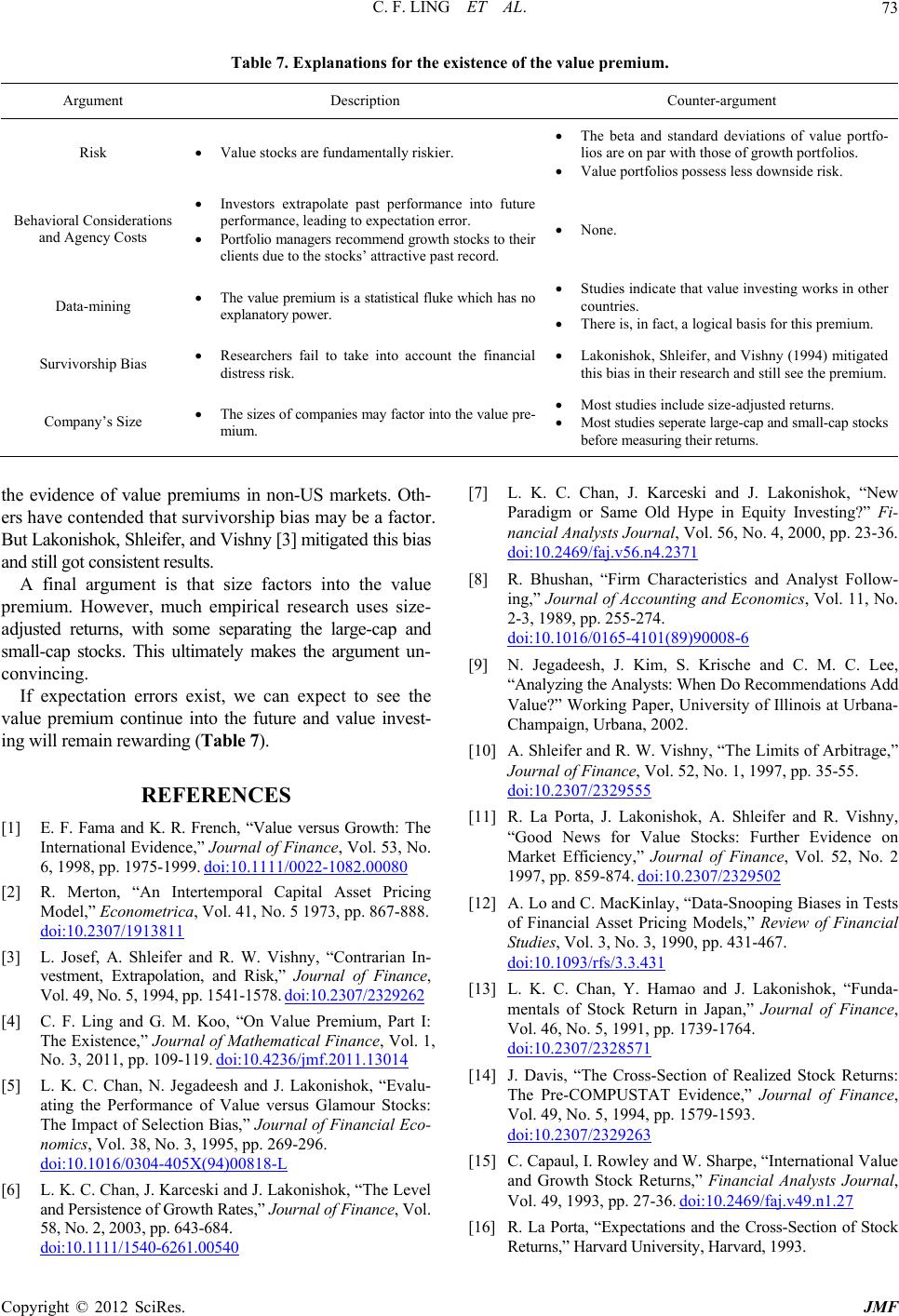. F. LING ET AL. 73
Table 7. Explanations for the existence of the value premium.
Argument Description Counter-argument
Risk  Value stocks are fundamentally riskier.
 The beta and standard deviations of value portfo-
lios are on par with those of growth portfolios.
 Value portfolios possess less downside risk.
Behavioral Considerations
and Agency Costs
 Investors extrapolate past performance into future
performance, leading to expectation error.
 Portfolio managers recommend growth stocks to their
clients due to the stocks’ attractive past record.
 None.
Data-mining  The value premium is a statistical fluke which has no
explanatory power.
 Studies indicate that value investing works in other
countries.
 There is, in fact, a logical basis for this premium.
Survivorship Bias  Researchers fail to take into account the financial
distress risk.
 Lakonishok, Shleifer, and Vishny (1994) mitigated
this bias in their research and still see the premium.
Company’s Size  The sizes of companies may factor into the value pre-
mium.
 Most studies include size-adjusted returns.
 Most studies seperate large-cap and small-cap stocks
before measuring their returns.
the evidence of value premiums in non-US markets. Oth-
ers have contended that survivorship bias may be a factor.
But Lakonishok, Shleifer, and Vishny [3] mitigated this bias
and still got consistent results.
A final argument is that size factors into the value
premium. However, much empirical research uses size-
adjusted returns, with some separating the large-cap and
small-cap stocks. This ultimately makes the argument un-
convincing.
If expectation errors exist, we can expect to see the
value premium continue into the future and value invest-
ing will remain rewarding (Table 7).
REFERENCES
[1] E. F. Fama and K. R. French, “Value versus Growth: The
International Evidence,” Journal of Finance, Vol. 53, No.
6, 1998, pp. 1975-1999. doi:10.1111/0022-1082.00080
[2] R. Merton, “An Intertemporal Capital Asset Pricing
Model,” Econometrica, Vol. 41, No. 5 1973, pp. 867-888.
doi:10.2307/1913811
[3] L. Josef, A. Shleifer and R. W. Vishny, “Contrarian In-
vestment, Extrapolation, and Risk,” Journal of Finance,
Vol. 49, No. 5, 1994, pp. 1541-1578. doi:10.2 307/2329 262
[4] C. F. Ling and G. M. Koo, “On Value Premium, Part I:
The Existence,” Journal of Mathematical Finance, Vol. 1,
No. 3, 2011, pp. 109-119. doi:10.4236/jmf.2011.13014
[5] L. K. C. Chan, N. Jegadeesh and J. Lakonishok, “Evalu-
ating the Performance of Value versus Glamour Stocks:
The Impact of Selection Bias,” Journal of Financial Eco-
nomics, Vol. 38, No. 3, 1995, pp. 269-296.
doi:10.1016/0304-405X(94)00818-L
[6] L. K. C. Chan, J. Karceski and J. Lakonishok, “The Level
and Persistence of Growth Rates,” Journal of Finance, Vol.
58, No. 2, 2003, pp. 643-684.
doi:10.1111/1540-6261.00 540
[7] L. K. C. Chan, J. Karceski and J. Lakonishok, “New
Paradigm or Same Old Hype in Equity Investing?” Fi-
nancial Analysts Journal, Vol. 56, No. 4, 2000, pp. 23-36.
doi:10.2469/faj.v56.n4.2371
[8] R. Bhushan, “Firm Characteristics and Analyst Follow-
ing,” Journal of Accounting and Economics, Vol. 11, No.
2-3, 1989, pp. 255-274.
doi:10.1016/0165-4101(89)90008-6
[9] N. Jegadeesh, J. Kim, S. Krische and C. M. C. Lee,
“Analyzing the Analysts: When Do Recommendations Add
Value?” Working Paper, University of Illinois at Urbana-
Champaign, Urbana, 2002.
[10] A. Shleifer and R. W. Vishny, “The Limits of Arbitrage,”
Journal of Finance, Vol. 52, No. 1, 1997, pp. 35-55.
doi:10.2307/2329555
[11] R. La Porta, J. Lakonishok, A. Shleifer and R. Vishny,
“Good News for Value Stocks: Further Evidence on
Market Efficiency,” Journal of Finance, Vol. 52, No. 2
1997, pp. 859-874. doi:10.2307/2329502
[12] A. Lo and C. MacKinlay, “Data-Snooping Biases in Tests
of Financial Asset Pricing Models,” Review of Financial
Studies, Vol. 3, No. 3, 1990, pp. 431-467.
doi:10.1093/rfs/3.3.431
[13] L. K. C. Chan, Y. Hamao and J. Lakonishok, “Funda-
mentals of Stock Return in Japan,” Journal of Finance,
Vol. 46, No. 5, 1991, pp. 1739-1764.
doi:10.2307/2328571
[14] J. Davis, “The Cross-Section of Realized Stock Returns:
The Pre-COMPUSTAT Evidence,” Journal of Finance,
Vol. 49, No. 5, 1994, pp. 1579-1593.
doi:10.2307/2329263
[15] C. Capaul, I. Rowley and W. Sharpe, “International Value
and Growth Stock Returns,” Financial Analysts Journal,
Vol. 49, 1993, pp. 27-36. doi:10.2469/faj.v49.n1.27
[16] R. La Porta, “Expectations and the Cross-Section of Stock
Returns,” Harvard University, Harvard, 1993.

C. F. LING ET AL. 74
[17] R. Banz and W. Breen, “Sample Dependent Results Us-
ing Accounting and Market Data: Some Evidence,” Jour-
nal of Finance, Vol. 41, No. 4, 1986, pp. 779-793.
doi:10.2307/2328228
[18] S. P. Kothari, J. Shanken and R. Sloan, “Another Look at
the Cross-section of Expected Stock Returns,” University
of Rochester, Rochester, 1992.
[19] R. W. Banz, “The Relationship between Return and Mar-
ket Value of Common Stock,” Journal of Financial Eco-
nomics, Vol. 9, No. 1, 1981, pp. 3-18.
doi:10.1016/0304-405X(81)90018-0