Journal of Mathematical Finance, 2012, 2, 13-30
http://dx.doi.org/10.4236/jmf.2012.21002 Published Online February 2012 (http://www.SciRP.org/journal/jmf)
A Comparison of VaR Estimation Procedures for
Leptokurtic Equity Index Returns*
Malay Bhattacharyya1, Siddarth Madhav R2
1Indian Institute of Management Bangalore, Bangalore, India
2Barclays Capital, New York, USA
Received July 11, 2011; revised August 1, 2011; accepted August 29, 2011
ABSTRACT
The paper presents and tests Dynamic Value at Risk (VaR) estimation procedures for equity index returns. Volatility
clustering and leptokurtosis are well-documented characteristics of such time series. An ARMA (1, 1)-GARCH (1, 1) ap-
proach models the inherent autocorrelation and dynamic volatility. Fat-tailed behavior is modeled in two ways. In the
first approach, the ARMA-GARCH process is run assuming alternatively that the standardized residuals are distributed
with Pearson Type IV, Johnson SU, Manly’s exponential transformation, normal and t-distributions. In the second ap-
proach, the ARMA-GARCH process is run with the pseudo-normal assumption, the parameters calculated with the
pseudo maximum likelihood procedure, and the standardized residuals are later alternatively modeled with Mixture of
Normal distributions, Extreme Value Theory and other power transformations such as John-Draper, Bickel-Doksum,
Manly, Yeo-Johnson and certain combinations of the above. The first approach yields five models, and the second ap-
proach yields nine. These are tested with six equity index return time series using rolling windows. These models are
compared by computing the 99%, 97.5% and 95% VaR violations and contrasting them with the expected number of
violations.
Keywords: Dynamic VaR; GARCH; EVT; Johnson SU; Pearson Type IV; Mixture of Normal Distributions; Manly;
John Draper; Yeo-Johnson Transformations
1. Introduction
VALUE AT RISK (VaR) is a popular measure of risk in
a portfolio of assets. It represents a high quantile of loss
distribution for a particular horizon, providing a loss thresh-
old that is exceeded only a small percentage of the time.
Traditional methods of calculating VaR include his-
torical simulation and the analytic variance-covariance
approach. However, these models fall short when tested
against actual market conditions. The historical simulation
approach assumes constant volatility of stocks over an
extended period of time. It fails to account for the phe-
nomenon of volatility clustering, when periods of high
and low volatility occur together. This leads to underes-
timation of VaR during periods of high volatility, and
overestimation in times of calm. The analytic variance-
covariance approach assumes that returns are jointly nor-
mally distributed. However, the fat-tailed non-normal be-
haviour of returns would mean that this methodology tends
to underestimate VaR as well.
Fama [1] and Mandelbrot [2] report the failure of the
normal distribution to model asset returns, sparking a slew
of papers addressing the issue of accurately modeling lep-
tokurtic time series with volatility clustering. The ap-
proaches can be roughly divided in two, the first assuming
that returns are independent and modeling unconditional
distribution of returns. In this approach, numerous distri-
butions have been proposed, Fama [1] and Mandelbrot [2]
use the stable Paretian distribution, Blattberg and Gonedes
[3] suggest the use of Student t-distribution. The mixture
of normal distributions is used by Ball and Torous [4]
and Kon [5] and the logistic distribution, the empirical
power distribution and the Student t-distributions have
been compared by Gray and French [6]. The Pearson type
IV distribution is used by Bhattacharyya, Chaudhary and
Yadav [7] for dynamic VaR estimation and by Bhat-
tacharyya, Misra and Kodase [8] for dynamic MaxVaR
estimation. Bhattacharyya and Ritolia [9] use EVT for
dynamic VaR estimation.
The second approach considers returns to be serially
correlated and uses conditional variance models or sto-
chastic volatility models to model asset returns. Engle
[10] and Bollerslev [11] use ARCH and GARCH models
to account for volatility clustering. GARCH models have
*This work was carried out when Siddarth Madhav R was a graduate
student at the Indian Institute of Management Bangalore.
C
opyright © 2012 SciRes. JMF

M. BHATTACHARYYA ET AL. 14
been shown to be more suited to this purpose by various
studies such as Poon and Granger [12]. The GARCH (1,
1) model performs well for most stock returns and this
paper adopts this approach.
The following model has been extensively used to
model dynamism in forecasts of returns and volatility of
returns.
tttt
X
Z

  (1)
where t
X
is the actual return on day t, t

is the ex-
pected return on day t, t

is the volatility estimate on
day t and t
Z
is the standardized residual, having a nor-
mal distribution with zero mean and unit standard devia-
tion.
ARMA processes are useful for modeling t

, the
predicted mean of the time series data, and GARCH
processes are good models for t

, the predicted volatile-
ity. However, the inherent leptokurtic behaviour of asset
returns makes the ARMA-GARCH model insufficient
for the purpose of calculating VaR.
In this paper, ARMA (1, 1) model is used for the cal-
culation of predicted mean and GARCH (1, 1) model is
used for modeling the observed volatility clustering.
Models are developed using two approaches. In the first
one, consisting of five models, ARMA-GARCH model
parameters are calculated assuming that standardized
residuals alternatively follow Pearson Type IV distribu-
tion, Johnson U distribution, Manly’s exponential trans-
formation, normal and Student t-distributions. In the
second approach, the ARMA-GARCH parameters are
calculated using the pseudo-normal assumption, i.e., as-
suming that standardized residuals are normally distrib-
uted, and they are later modeled using the mixture of
normal distributions, Extreme Value Theory, and other
power transformations such as John-Draper, Bickel-
Doksum, Manly, Yeo-Johnson and certain combinations
of the above. The second approach yields nine models.
S
While developing and testing VaR models, the authors
find it important to develop those that are applicable in
real world scenarios. This translates to certain simplicity
in execution and fast run-times for calculations, as time
can be a critical issue. At the same time, the importance
of creating an accurate measure of risk cannot be under-
stated, given how the stock market crash of 2008 bank-
rupted firms and individuals alike, and sent the world spi-
raling into recession.
2. Leptokurtic Density Functions
2.1. Pearson Type IV Distribution
The Pearson family of curves, a generalized family of fre-
quency curves developed by Karl Pearson, embodies a
wide range of commonly observed distributions. The Pear-
son curves are a solution to the differential equation



2
01 2
d
1
d
fx x
fx x ccxcx
 
 (2)
The system of curves which arise from the above dif-
ferential equation cover a wide spectrum of skewness
and kurtosis (Figure 1). The type of distribution obtained
post-integration is dictated by the roots of the quadratic
equation 2
01 20ccxcx

.
The Type IV curve is obtained when the roots of the
quadratic equation 2
01 20ccxcx

 are complex, i.e.,
when 2
. It is suitable for those distributions
which have high excess kurtosis and moderate skewness.
Financial return data fall in this category. The probability
density function (PDF) of the Type IV curve (Heinrich,
[13]) is
2
10
4ccc

2
1
1exptan
m
xx
fx kaa








 
 

  
 
 



(3)
where λ, a, ν and m are real parameters (functions of α,
), m > 1/2,
01 2
, and cc c
x

  and k is a norma-
Figure 1. The diagram of the Pearson curve family. It shows
the type of curve to be used for each range of skewness and
kurtosis. The x-axis is β1 = skewness2, and the y-axis is β2,
the traditional kurtosis.

M. BHATTACHARYYA ET AL. 15

lizing constant, dependent on λ, a, ν and m. ARCH process, we require a transformation function which
can accept arguments that may be positive or negative.
Hence we need to use the Johnson U distribution, as the
sine hyperbolic inverse function has a domain all over the
real line.
S
The PDF gives rise to a bell shaped curve, where λ is
the location parameter, a is the scale parameter, ν and m
can be interpreted as the skewness and kurtosis parame-
ters respectively.
The type of Pearson curve to use for a particular situa-
tion is dictated by the skewness and kurtosis. Table 1
shows the observed skewness and excess kurtosis for the
six equity indices. Cross-referencing them with Figure 1,
we can see that Pearson Type IV curve is the model to be
used.
So we have
1
*sinh X Z

 


 



(7)
where

and

are assumed to be positive.
The density function of Johnson U distribution can
be easily found in closed-form from variable transforma-
tion:
S
For a standardized Pearson Type IV curve, i.e., with
zero mean and unit standard deviation, we need to add the
following constraints.

1
2
;;;; sinh
1
x
fx
x








 







(8)

2
22
1
s
rr
ar


 (4)
sar

  (5)
where
x
R

,

is the density function of , (0,1)N

and

> 0 are location and scale parameters respect-
tively,

can be interpreted as a skewness parameter,
and

> 0 can be interpreted as a kurtosis parameter.
The distribution is positively or negatively skewed ac-
cording to whether

is negative or positive. Holding

constant and increasing

reduces the kurtosis. How-
ever,

and

cannot be viewed purely as skewness or
kurtosis parameters, respectively. The mean and the
variance of Johnson SU distribution are given as:
2.2. Johnson SU Distribution
The Johnson family of distributions (Johnson, [14]) con-
sists of three distributions, which cover all possible av-
erage, standard deviation, skewness and kurtosis values,
excluding the impossible region. These consist of the
UB
and the lognormal curves. The transformations
have the general form
S,S
.X Zg

 


 



(6)
12sinh Ω
  (9)
where the transformation parameters ξ is the location, λ is
the scale and γ and δ are shape parameters. Z is the re-
sulting normal distribution.


.
g
is one of the following
functions:

2
21ccosh2Ω1
2




 (10)
where


2
exp 

 and

  .




1
U
B
ln Lognormal distribution
sinh Sdistribution
ln1 Sdistribution
Normal distribu ton i
y
gy
y
y
y
y








2.3. Extreme Value Theory
Extreme value theory provides a framework to formalize
the study of behavior in the tails of a distribution. Ac-
cording to the Fisher-Tippet theorem, there can be three
possible extreme value distributions for the standardized
variable.
Since we are modeling the innovations of the ARMA-
Table 1. Comparison of moments for each stock index return series.
Index Sensex NIFTY DJI FTSE HSI Nikkei
Observations 1500 1500 1500 1500 1500 1500
Dates Mar 03 - Feb 09 Mar 03 - Feb 09Mar 03 - Feb 09Mar 03 - Feb 09Mar 03 - Feb 09 Mar 03 - Feb 09
Mean 0.0009 0.0009 0.0001 0.0002 0.0004 0.0001
Std. Deviation 0.0178 0.0181 0.0124 0.0127 0.0169 0.0163
Skewness −0.4276 −0.5130 0.2624 0.1409 0.3876 −0.2730
Kurtosis 7.2358 8.6112 17.3926 14.5248 15.5344 12.8085

M. BHATTACHARYYA ET AL. 16
2.3.1. Gumbel Distrib ut ion
As with the normal and gamma distributions, the tail can
be unbounded, have finite moments and decay exponent-
tially. The distribution function is given by:


expe for
x
Gx x



(11)
2.3.2. Frechet Distribution
The tail can be unbounded, and decay by a power as with
the Cauchy and Student t-distribution. The distribution
function is given by


0 for 0
exp for 0
x
Gx xx
 






(12)
Moments exist only up to the integer part of α, higher
moments do not exist, as the tails are fat, they are not
integrable when weighted by tail probabilities.
2.3.3. Wei b ull Distribution
The tails are constant-declining, and all moments exist.
They are thin, and have upper bounds. The distribution
function is:
 

exp for 0
1 for 0
xx
Gx
x

 




(13)
Now, since the financial returns data are fat-tailed and
unbounded, we must clearly use the Frechet distribution
for modeling extreme value distributions.
2.3.4. Generalized Extreme Value Distribution
The Generalized Extreme Value Distribution (GEVD)
unifies the above three distributions. Here the tail index
(τ) is the inverse of the shape parameter (α). In this equa-
tion given below, if 0

, it is a Gumbel distribution, if
0

, it is a Frechet distribution else if 0

 it is a
Weibull distribution.
 


1/
exp1 for 0
exp for 0
xx
x
Fx
e





 




(14)
To build the series of maxima or minima, there are two
methods:
2.3.5. Block Maxima
This approach consists of splitting the series into equal
non-overlapping blocks. The maximum from each block
is extracted and used to model the extreme value distri-
bution. As volatility clustering is a well observed pheno-
menon in financial data, very high or very low observa-
tions tend to occur together. Thus, this technique runs the
2.3.6. Pe ak over Thresh ol d
risk of losing extreme observations.
of sampling maxima by se-
2.4. Mixture of Normal Distributions
o model fat-
The second approach consists
lecting those that exceed a chosen threshold. A low thres-
hold would give rise to a larger number of observations,
running the risk of including central observations in the
extremes data. The tail index computed has lesser vari-
ance but is subject to bias. A high threshold has few ob-
servations, and the tail index is more imprecise, but un-
biased. The choice of the threshold is thus a trade-off be-
tween variance and bias. For the analysis in this paper,
we use the Peak over Threshold method.
The mixture of normal distributions, used t
tailed distributions, assumes that each observation is gen-
erated from one of N normal distributions. The probabil-
ity that it is generated from a distribution “i” is i
p, with
11
N
i
ip 

.
The resultant density function
 
112 2
1
;
N
NN ii
i
x
pppp x  


 (15)
where is a normal distribution with mean i

i

and
standareviation i d d

. For the special case of 2N

,
we have




1
;1
2
x
pxp x     (16)
where


1212
,, ,,p

  
mixture of N normal
is the parameter vector.
ur
m
For a distributions, the first fo
oments are:
1
N
ii
i
p




 (17)
2222
11
NN
ii ii
ii
pp







 (18)

23 23
3
1
133
N
ii i
i

 


 









 (19)

422
4
1
3224
136
46
N
iiii i
i
p



4



 










(20)
A mixture of more than two normal distributions may
provide a better fit to the series, but Tucker [15] reports
that the improvement by increasing the number of nor-
mal distributions in the mixture from two is not too sig-
nificant. Estimation of parameters for the mixture of nor-
mal distribution is problematic. This is because, although
we have a well defined distribution function in a closed
form, using maximum likelihood techniques for parame-
ter estimation leads to convergence issues (Hamilton, [16]).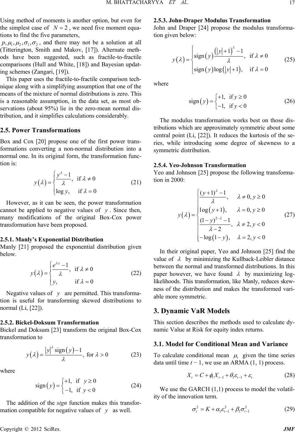

M. BHATTACHARYYA ET AL. 17
Using method of moments is another option, but even for
the simplest case of 2N, we need five moment equa-
tions to find the five pters,
1212
,, ,,p
arame

 , and there may n
mith and Makov, [17]). Alternate meth-
ods have been suggested, such as fractile-to-fractile
comparisons (Hull and White, [18]) and Bayesian updat-
ing schemes (Zangari, [19]).
This paper uses the fractile
ot be a solution at all
-to-fractile comparison tech-
ni
2.5. Power Transformations
f the first power trans-
(Titterington, S
que along with a simplifying assumption that one of the
means of the mixture of normal distributions is zero. This
is a reasonable assumption, in the data set, as most ob-
servations (about 95%) lie in the zero-mean normal dis-
tribution, and it simplifies calculations considerably.
Box and Cox [20] propose one o
formations converting a non-normal distribution into a
normal one. In its original form, the transformation func-
tion is:

1, if 0
log, if 0
y
y
y









(21)
However, as it can be seen, the power transformation
ca
ox
2.5.1. Manly ’s Exp onen ti al Di stri bution
ibution given
nnot be applied to negative values of y. Since then,
many modifications of the original B-Cox power
transformation have been proposed.
Manly [21] proposed the exponential distr
below.

1, if 0
, if 0
y
e
y
y









(22)
Negative values of are permitted. This transforma-
tio sf
2.5.2. Bickel-Doksum Transformation
iginal Box-Cox
y
n is useful for tranorming skewed distributions to
normal (Li, [22]).
Bickel and Doksum [23] transform the or
transformation to
 
sign 1, for 0 yy
y




   (23)
where
(24)
The addition of the sign function makes this transfor-
m
at
John and Draper [24] propose the modulus transforma-

1, if 0
sign 1, if 0
y
yy




ation compatible for negative values of y as well.
2.5.3. John-Dr aper M odul u s Transformion
tion given below:
 

 
11
sign, if 0
signlog1, if 0
y
y
y
yy





 



(25)
where

1, if 0
sign 1, if 0
y
yy






 (26)
The modulus transformation works best
tributions which are approximately symmetric about some
ce
nsformation
Yeo and Johnson [25] propose the following transforma-
on those dis-
ntral point (Li, [22]). It reduces the kurtosis of the se-
ries, while introducing some degree of skewness to a
symmetric distribution.
2.5.4. Yeo- Johnson Tra
tion in 2000:
 

2
(1)1
, 0,0
log1, 0,0
(1)1, 2,0
2
log1, 2,0
yy
yy
yyy
yy










 



 









(27)
In their original paper, Yeo and Johnson [25] find the
value of

by minimizing the Kullback-Leibler distance
between the normal and transformed distributions. In this
paper however, we have found

by maximizing log-
likelihoods. This transformation, like Manly, reduces skew-
ness of the distribution and makes the transformed vari-
able more symmetric.
3. Dynamic VaR Models
s used to calculate dy-
x returns.
ariance
This section describes the method
namic Value at Risk for equity inde
3.1. Model for Conditional Mean and V
To calculate conditional mean t

given the time series
data until time t − 1, we use an ARMA (1, 1) process.
1111tttt
XC X

 


 (28)
We use the GARCH (1,1) process to m
ity of the innovation term.
t
odel the volatil-
222
11 t
K1 1
t

   

(29)

M. BHATTACHARYYA ET AL. 18
3.2. Models for Innovations
In Equation (1), the forecasted mean and variance are
ARCH (1, 1) model. As
pr
calculated by an ARMA (1, 1)-G
mentioned in the introduction, there are two approaches
followed to model innovations. In the first approach,
ARMA (1, 1)-GARCH (1, 1) model parameters are cal-
culated assuming that standardized residuals alternatively
follow Pearson Type IV distribution, Johnson U
S dis-
tribution, Manly’s exponential transformation, normal
and Student t-distributions. In the second apoach,
ARMA (1, 1)-GARCH (1, 1) parameters are calculated
assuming that standardized residuals are normally dis-
tributed. The extracted standardized residuals are then
modeled using the mixture of normal distributions, Ex-
treme Value Theory, and other power transformations such
as John-Draper, Bickel-Doksum, Manly, Yeo-Johnson and
certain combinations of the above.
Method 1
The first approach consists of five models, whose de-
sined below. gns are outli
Model 1.1 GARCH-N Model
In Equation (1), t
Z
is assumed to be a standard nor-
mal distribution. Therefore, the innovations term, , has
ze
t

ro mean and the standard deviation of t h.
 
0,1 0,
ttt
Z
NNh 
(30)

2
1

1
|e xp
2
2π
t
tt
t
t
fF h
h




Therefore, the log likelihood function
mized to find the parameters of the
m

(31)
, which is maxi-
ARMA-GARCH
odel for the series of length T is given by

2
1
1log 2π
22
T
t
t
tt
LLFh h


 




(32)
The maximum likelihood estimates for
1)-GARCH (1, 1) parameters are found
th
the ARMA (1,
by minimizing
e negative of the above function using the fmincon func-
tion in MATLAB.
Model 1.2 GARCH-t Model
In Equation (1), t
Z
is assumed to be a Student t-dis-
tribution with zero mean and unit standard deviation. There-
fore, the log likeliho function, the logarithm of the den-
sity function of the innovations term, t
 , for the series of
length T is given by
od




1
2
1
Γ
log
T
LLF









1 2log
2
Γπ2
2
1
log1
22
t
t
t
t
h
h


















 


 


 


(33)
where represents the degrees of freedom in the t-dis-
tribution.
The maximum likelihood estimates for the ARMA (1,
1) GARCH (1, 1) parameters are found by minimizing
the negative of the above function using the fminco
tion in MATLAB.
Model 1.3 GARCH-PIV Model
In Equation (1),
n func-
t
Z
is assumed to be a Pearson Type
IV distribution. Thandardized innovations series has
ia
e,
e st
unit varnce, but not necessarily a zero mean. This was
justified by Newey and Steigerwald [26], who proved that
an additional location parameter is needed to satisfy the
identification condition for the consistency of parameter
estimates when conditional innovation distribution in the
GARCH model is asymmetric. Hence Equation (4) holds,
but Equation (5) does not. Therefor

1
s
t
tt t
a
EX Fhr




 


(34)
Hence, for modeling innovations, we need to change
the location and scale parameters to t h  and
s
t
ah
respectively. The normalizing parameter is inversely pro-
portional to the scale parameter, so it changes to t kh.



,,, ,
ts
ZPIVkma  
,,, ,
tt stt
PIV kh mahh   
(35)
The distribution function of the innovation series is
given by

2
1tt
h
k
fF





 
1tt
ts t
ha h




1
exp tan
m
tt
st
h
ah



















(36)

The log likelihood function to be maximized is given
by





1
222
2
22
1
2
12
log log
22
log11
tan
1
T
t
t
tt
t
tt
t
r
LLFkh
hr
rr h
hr
rr
v
v
v
h

































(37)
We use Equation (4) and the relation


21rm
to
write
s
a
s ma
and in terms of . The log lic-
tion ixim(by minimng –LLF n-
m
ized
r
izi
kelihood fun
) using the fmi

M. BHATTACHARYYA ET AL. 19
con function in MATLAB. The maximum likelihood
estimates from the GARCH-N model and the Pearson
Type IV parameters calculated from the first four mo-
ments of the resulting standardized innovations series
(under the pseudo-normal assumption) are used as initial
estimates for the optimization function. Th
constant k is computed by the technique use
[13].
Model 1.4 GARCH-JSU Model
In this model, the standardized innovations in Equa-
tion (1),
e normalizing
d by Heinrich
t
Z
with
is assumed to be a Johnson distribu-
tion. As the GARCH-PIV model, thandardized
inecessarily z
U S
e st
novations have unit variance, but not nero
mean. Therefore, from Equation (10), the scale parameter
λ is constrained.
 
2
1coshcosh2Ω1
s
  (38)
where

2
exp 

 and Ω



.
Note that Equation (9) does not hold, and the parame-
ter ξ has to be estimated during optimization. The pre-
dicted future value of the time series is given by



12sinh Ω
 (39)
1t tt t
EX Fh 
 
Now, for modeling the innovations series t  , the loca-
tion and scale parameters must be changed to t h  and
s
t
h  .


,,,
ts
t
ZJSU
,,,
t st
J
SUh h   
 
 
(40)

12
1
sinh
st
tt
h
h
h
1
st
h
tt
tt
st
fF
h













wh
e


 










(41)
ere
The log likelihood function to be maximizd is given
by

0, 1N  .

1
2 (42)
21
1
loglog 2π
2
11
log1sinh
22
T
st
t
tt
LLF logh 







 


The maximum likelihood estimates are calculated by
minimizing the negative of the above function using the
fmincon function in MATLAB.
Model 1.5 GARCH-Manly Model
In this model, the standardized innovations in Equation
(1), it is assumed that when t
Z
is put through Manly’s ex-
ponential transformation (Equation (22)), it becomes nor-
mally distributed. Assuming that the transformed normal
function has zero mean and unit standard deviation, t
Z
c- has the following closed form probability distribution fun
tion


2
1
, 2π
exp 2
1
12
t
tt t
MZ
fZF Z
erf





 





(43)
where


,t
M
Z  is the exponentially transformed (Equa-
tion (22)) value of t
Z
and erf is the error function.
Therefore the standardizenovations ( have
following distribution
d int  the


1
expexp
2
t
t
h
11
1e rf2
tt
t
h
2
2
π
fF
exp 1
x
x
h























 









The log likelihood function to be maximized is given
by
(44)
1
2
2 






(45)
2
,
1
log2π
22
t
t
Mh 




2
log 1
1
T
t
t
t
t
LLF
erf
hh 


















The maximum likelihood estimates are calculated
minimizing the negative of the above function using
fmincon function in MATLAB. The above equation
derived in detail in the Appendix.
Method 2
The second approach consists of nine models, whose de-
signs are outlined below.
Model 2.1 GARCH-EVT Model
In this model, the ARMA (1, 1)-GARCH(1, 1)
m
at the standardized innovations in Equation (1)
by
the
para-
t
s are
eters are found under the pseudo-normal assumption,
i.e., th
Z
ade is a standard normal function. Now, the assumption m
is that the values of t
Z
considered for calculation
VaR, i.e., the 99th, 97. and 95th percentiles are pa
an extreme value distribution. This assumption is th
retically justified, as the ARMA-GARCH process gets rid
of
rt of
eo-
5th

M. BHATTACHARYYA ET AL. 20
of the serial correlation between terms, and the Fisher-
Tippet theorem is applicable.
We use the Peak over Threshold (POT) method to ob-
serve the number of values which exceed a high thresh-
old. The distribution of conditional excess losses over a
certain high threshold follows a Generalized P
tribution (GPD).
is the number atbove the threshol.
Therefo, the tail estimator becomes
of observions ad u
re

1
11, for
u
Nxu
F
xx
N



 u

 

 (49)
areto Dis-

11
q
u
N
VaR uq
N












 




(50)
The Value at Risk is now calculated by the formula
q
(51)
Choosing the threshold to be used in the calculations is
a subjective process. In this paper, we calculate the mean
excess returns for various values of thresholds and plot
them. For a GPD, the mean excess return is given by:

1
,
11, 0
1exp, 0 

 



where
x
Gx
x






  


 (46)

is the shape parameter (positive in our specific
case, as this yields a heavy tailed
q
ttt
VaR VaR  
GPD) and

is the
sceter.
he negative of the return series,
th is positive, and mean
ex
aling param
The formula for conditional excess losses above the
threshold u (We consider t

1
u
eu




 (52)
The threshold is calculated by observing the graphs
and identifying the point from which the conditional ex-
cess return increases linearly with the threshold values. It
is possible to consider any larger value as a threshold as
well, but this way, the maximum number of data points
gets accommodated in the extreme value distribution,
thus reducing the variance of the obtained parameters. In
Figures 2(a) and (b), we observe that the thresh old
ereby ensuring that the threshold
cess return is positive) is given by
 
|
u
F
yPXyuXu (4)
  
7
 
1
u
F
yF yuFuFu (48)
Since

u
F
y is a GPD with positive

, we need to
back-calculate

F
yu.


F
u is given by u NN,
where N is the total number of observations and u N
Figure 2. The optimal threshold is calculated by plotting the mean excess function of the six time series. The point is chosen at
thwhere w seen, the DJI graph is an anomaly, where no such clear point is
pres
e point the graph begins to slope upards. As can be
ent.

M. BHATTACHARYYA ET AL. 21
value for Sensex returns is at 1.4, and for Nifty, it is at
1.5. Note that in the graphs, we consider the negative of
the return series, which is why the threshold values are
positive.
For certain time series, the graph obtained
useful for finding the threshold. Consider the mean ex-
cess return for DJI in Figure 2 for instance.
we consider an appropriately high value fo
such as the 95th percentile of negative returns.
sumption to calculate the ARMA (1
parameters. The standardized innovations are assumed to
ha
ese standardized innovations.
The mean of one of the two normal distributions in the
mixture is assumed to be zero. This assumption is rea-
sonable, as results show that the probability that the stan-
dardized residuals lie in this normal distribution is very
high. A small percentage lies in the other distribution, with
the non-zero mean and higher variance, these yield the
very high and very low values observed in the data.
Thus, the parameter vector is of size four:
is not very
In such cases,
r the threshold,
Model 2.2 GARCH-MixNorm Model
This model also makes use of the pseudo-normal as-
, 1)-GARCH (1, 1)
ve a mixture of two normal distributions. We calculate
the mean, standard deviation, skewness and kurtosis of
th

112
,,,p

 .
point lies in the first (no
p is the probability that the data
n-zero mean) distribution, 1

is
distribution, the mean of the first 1

and 2

are
butio
the
the first anond ns
respectively. The mean of the second distribution is as-
sumed to be zero.
The parameter vector components must satisfy the four
moment constraints.
standard deviations ofd secdistri
1ep

 (53)

22 22
12
1
11
ee
pp p  

 


(54)

22 2
1
32
31
e
eee
ep
 

 
 


(55)
1




2
4 1
eee e

 



is possible
th if the first five
m
di-
vided into seven sets; less than 0.5 standard deviations,
0.5 – 1, 1 – 1.5, 1.5 – 2, 2 – 2.5,
3 standard deviations. The actual number of residuals in
ea
44 22 1
12
4
34
1331 6
1
eee
e
pp p

 









(56)
3
p


An obtained solution is feasible if it satisfies the con-
straints 22
12
0, 0   and 01p.
To calculate the parameters through the method of
moments, we need five moment equations. It
at there may not be a solution even
oments were calculated. So we employ a fractile-to-
fractile comparison test in addition to using certain mo-
ment equations.
We employ a modified version of the technique used
by Perez [27]. The data (standardized residuals) is
2.5 – 3, and greater than
ch category


k

is compared with the predicted
number of residuals for the solution each obtained from
the moment equations


k
 . The solution considered is
the one obtained by maximizing the log likelihood function


7
1
,log
kk
k
L 

  (57)
and satisfying the constraint Equations (49), (50), (52)
and (53). As it turns out in most cases, there is no solu-
tion which satisfies all of them, in such cases, constraint
Equation (52) is dropped. The minimization is carried out
using the fmincon function in MATLAB. It turns out that
the optimum values of the parameter are dependent on
the initial values considered, so the parameters obtained
for the previous data point are used as initial values in the
optimization for the next one.
The Value at Risk is now calculated by the formula in
Equation (48), where is calculated from inserting
the calculated param mixture of normals
probability density function given by Equation (16) and
cumulating it by numerical methods.
Model 2.3 GARCH-Bickel-Doksum Model
We calculate the ARMA (1, 1)-GARCH (1, 1) parame-
ters under the pseudo-normal assumption. The standard-
ized residuals obtained
q
t
VaR
eters in the


t

Bickel and
(23) an
rame
are put through the trans-
formation suggested by Doksum [23] to nor-
malize them (Equationsd (24)). If we assume that
for some value of the pater

, the transformed ob-
servations


,i T  ributed with mean are normally dist

and statandard deviion

. The parameter is esti-
mated by maximizing the log likelihood function





2
2
2
1
|log2π,
22
t
ti
n
lT
1i
1
1log
t
i
i



 


 (58)





where


,,

 . The maximum likelihood estimate
for the mean and variance is given by


1
1
ˆ,
t
i
i
T
t
 

 
(59)
  
(60)
The estimate for

2
21
ˆˆ
,
t
i
T   


1
i
t

can, therefore, be obtained by
simply maximizing the likelihood function

M. BHATTACHARYYA ET AL. 22



2
ˆ |log2π1log
2
ti
n
l     (61)
As shown in Table 2(a), the Bickel-Doksum transfor-
mation does not handle skewed distributions well, as it
only reduces kurtosis. Hence, this model must be modi-
fied to fix this drawback.
The Value at Risk is now calc
Equation (48), whereis calculated from the in-
verse Bickel-Doksum
ulated by the formula in
q
t
VaR
formula



1
12
ˆˆ 11,,
q
t
VaRN q

 

  
 
(62)
where

12
ˆˆ
,,Nq

 


for probability

is the inverse
tion
normal func-

1q, mean

ˆ

 and variance

2
ˆ


Mo . del 2.4 GARCH-John-Drape
We calculate the ARMA (1, 1)-GARCH (1, 1) p
ters under the pseudo-normal assumption. The standard-
ized residuals obtainedare transformed with the mo-
dulus transformation ped by John and Draper [24]
(E
ious model, meter
r Model
arame-

t

ropos
th
quations (25) & (26)). By using similar arguments as
the preve para

is estimated by
maximizing the log likelihood function


 
2
1
ˆ
log 2π1log 1
2
t
ti
i
n
l 

 

 (63)
where 2
ˆ

is given by Equation (56) with

,i T   re-
presenting the modulus transformation.
ere
As with the Bickel-Doksum transformation, Table 2(a)
shows that the modulus transformation is not a skew-
corrector, it reduces kurtosis. Hence, this model must be
modified to correct this.
The Value at Risk is now calculated by the formula in
Equation (48), wh q
t
VaR is calculated from the in-
verse John-Draper formula
 


1
12
ˆˆ
111 ,,
q
t
VaRN q



 

(64)
where
 
12
ˆˆ
,,Nq

 


r probability

1q, m
is the inverse normal func-
tion foean

ˆ


 and variance

2
ˆ

 .
Model 2.5 GARCH-Yeo-Johnson Model
We calculate the ARMA (1, 1)-GARCH (1, 1) para-
meters under the pseudo-normal assumption. The stan-
dardized residuals obtained


t
 are transformed with
the Yeo-Johnson [25] transformation (Equations (27)). By
using similar arguments as the previous models, the pa-
rameter

is estimated by maximizing the log likeli-
hood function





1
ˆ
log 2π1signlog1
2
ti
i
i
l 

 


(65)
2 re-
Yeo-Johnson trans-
fo The model
m
2
nt
where ˆ

presenting the Yeo-Johnson transformation.
Tables 2(a) and (b) show that the
rmation is a skew-correcting transformation.
ust be modified to enable kurtosis-handling as well.
The Value at Risk is now calculated by the formula in
Equation (48), where V is calculated from the in-
verse Yeo-Johnson formula

q
t
aR



12
12
ˆˆ
1121,,
q
t
VaRN q




 

(66)
ere wh




12
ˆˆ
,,Nq

 




s the inverse normal func-
tion for probability
i


1q

, mean

ˆ

 and variance


2
ˆ


Mo . del 2.6 GARCH-Manly-Johnodel
We calculate the ARMA (1, 1)-GARCH (1, 1) und
pseudo-normal assumption. The innovations are initially
transformed through the Manly exponential transforma-
rid it of skewn
oubly-transformed
data obtained is now roughly normally distributed (Ta-
bles 2(a) and (b)).
To obtain the parameter for the Manly transformation,
the following log-likelihood function is maximized.
-Draper M
er the
tion toess. The symmetric data is now
transformed with the John-Draper modulus transforma-
tion, which reduces kurtosis. The d
 
2
1
2
ti
i
The parameter for the John-Draper tran
ˆ
log 2πλ
t
n
l     (67)
sformation is
obtained by maximizing the log-likelihood funct
Equation (60).
ion in
The inverse Manly transformation is given by
 
12
1ˆˆ
log 11,,
q
t
VaRNq 










 (68)
The Value at Risk is calculated in two steps. First, the
low quantile value is ected to the inverse John-
Draper transformation in Equat
subj
ion (61) and this value is
back-transformed with the inverse Manly transformation
in Equation (65).
2.7 GARCH-Manly-Bi
MA (
ption. vatio
tran sforma-
tio
he inverse trans-
formations in Equations (59) and (65) carried out serially
in that order.
Modelckel-Doksum Model
We calculate the AR1, 1)-GARCH (1, 1) under the
pseudo-normal assum The innons are initially
msfored through the Manly exponential tran
n remove skewness, and then with the Bickel-Doksum
transformation, which reduces kurtosis. The skewness and
kurtosis of the doubly-transformed insample data is given
in Tables 2(a) and (b).
The parameters for the Manly and Bickel-Doksum trans-
formations are calculated by maximizing log-likelihoods
in Equations (64) and (58). After the two parameters are
obtained, the VaR is calculated from t
is given by Equation (56) with


,i T 

M. BHATTACHARYYA ET AL. 23
Table 2. (a) Skewness comparison of std. residualser transformation; (b) Kurtosis comparison of std. residuals
after power transformation.
NIFTY
after pow
(a)
SensexDJI FTSE HSI Nikkei
Initial skewness −0.4764 −0.5311 −0.1024 −0.3660 −0.1836 −0.3209
Manly 0.0134 0.0615 0.0035 0.0162 0.0126 0.0072
−0.0801 −0.2763 −0.0815 −0.2299 John-Draper −0.3694 −0.2842
Yeo-Johnson 0.0037 0.0442
Bickel-Doksum
0.0094 0.0055 −0.0175 −0.0306
−0.0858 −0.3045 −0.1069 −0.2638−0.4379 −0.3769
Manly-Yeo-Johnson 0.0052 00.0093 0.0068 −0.0221
Manly-John-Draper −0.0026 0.0052 0.0226 0.0150
m 126
−0.0087
0130
0.0041 −0.0003 0.0026 −0.0193
.0356 −0.0287
0.0070 −0.0026
Manly-Bickel-Doksu0.00.0281 −0.0015 0.0068 0.0208 0.0123
0.0051 −0.0022 −0.0151 −0.0284 John-Draper-Yeo-Johnson −0.0063
Yeo-Johnson-John-Draper −0.0002 0.0028
Yeo-Johnson-Bickel-Doksum 0.0029 0.0233
0.0028 −0.0002 0.0088 −0.
The standardized residuals for the in-sample data are transformed with various
check their normalizing effect. For double-transformations, the data is first tra
ond transformation.
(b
power transformations. The skewness of each transformed output is co
nsformed with the transformation mentioned first, and then subjected to the sec-
)
Sensex NIFTY
mpared to
DJI FTSE HSI Nikkei
Initial kurtosis 3.7840 5.0195 3.3459 3.8574 3.9326 3.5752
Manly 3.3038 4.93
3.17
4.7952
72
3.2771 3.8375
John-Draper-Yeo-Johnson 2.9229 3.0349
Yeo-Johnson-John-Draper 3.1005 3.18
Johnson-Bickel-Doksum 3.1907 3.0305 3.0275
18 3.3380 3.4958 3.8097 3.1979
John-Draper 3.1862 18
Yeo-Johnson 3.3475
2.8817 3.1754 2.8691 3.0347
3.3385 3.5389 3.8324 3.2611
2.9518 3.3488 3.0716 3.2118
3.3388 3.4952 3.8182 3.2126
Bickel-Doksum 3.5532 3.8147
Manly-Yeo-Johnson 3.3032 4.89
Manly-John-Draper 3.0932 3.2107
Manly-Bickel-Doksum
2.8838 3.0976 2.8498 2.9224
2.9502 3.1660 3.0251 2.9903
2.8775 3.0082 2.8458 2.8674
2.8840 3.1073 2.8531 2.9431
2.9565
69
Yeo-3.2998 3.7688
The standardized residuals f-sample datansformed with variousor the in are tra power transformations. The kurtosis of each transformed output is compared to
check their normalizing effect. For double-transformations, the data is first transformed with the transformation mentioned first, and then subjected to the sec-
ond transformation.
Model 2.8 GARCH-Yeo-Johnson-John-Draper Model
We calculate the ARMA (1, 1)H (1, 1
the pseuption. Tvations-
tially traugh the Yon tra-
tion to rid it ness. The symmata is no-
formed whn-Draper mtransfo,
which reduces kursis. The doubed d-
tained is normally died (Tab
and (b)).
A the para for the two transform
obtfrom Eq (62) an the VaR-
p the iransfor in Equ1)
and (63). 2.9 GAo-Johnel-Doksum Model
We che (1, 1)(1, 1) unde
psormal an. Thtions ally
-GARC) under
do-normal assum
nsformed thro
he inno
eo-Johns
are ini
nsforma
of skewetric dw trans
ith the Jo
to
odulus
ly-transform
rmation
ata ob
now roughlystributles 2(a)
fter metersations are
ained
uted from
uations
nverse t
d (60),
mations
is com
ations (6
Model
alculate t
RCH-Ye
ARMA
son-Bick
-GARCH er th
eudo-nssumptioe innovare initia

M. BHATTACHARYYA ET AL. 24
transformhe Yeo-Johsform
removeen transfoith the Bicl-
Doksu which reexcess .
The skosis of tbly-tran
data o Tables (b).
Param-Johnsonickel-D
tran ted byizing l-
hood (58). The VaR is cad
frnverseationstions (59) and (63)
carri seriall order.
4. Testing
Tseries are of length 15se are diinto
thple serth 1000) and t-of-samies
(l00). Fdata pthe outple
rewe estiodel pars usinre-
Table 3. (a) 99% VaR violations comparisons for model 1 series; (b) 97.5% VaR violations comparisons for model 1 series; (c)
(a)
99% VaR Model 1.1 Normal 2 T Model 1.
n Type IV
Model 1.4
on SU 5 Manly Expected Violations
ed through tnson tranation to
skewness, and th
m transformation,
rmed w
moves
ke
kurtosis
ewness and kurthe dousformed
btained are given in2(a) and
eters for the Yeo
sformations are calcula
and B
maxim
oksum
og-likeli
ds in Equations (62) anlculate
om the i transform in Equa
ed outy in that
he data 00; thevided
e in-sam
ength 5
ies (leng
or each
ou
oint in
ple ser
-of-sam
gion, mate mrameteg the p
95% VaR violations comparisons for model 1 series.
Model 1.3
Pearso Johns Model 1.
Sensex 16 7 7 8 5 16
Nifty 16 8 8 13 5
DJI 22 20 9 9 11 5
FTSE 19 21 13 13 17 5
H S I 15 13 6 6 10 5
Nikkei 11 13 7 7 9 5
14
This tabletion comparisons f Model 1 see expectedf violations is gn in the last c 99% VaR is eted to
be violatnt out-of-samet. As can odels 1.3re the bestones.
(b)
9mal 1.2 T del 1.3
Pearson Type IV
odel 1.4
Johnson SU del 1.5 MExpected Violations
shows the VaR violaor theries. Th number oiveolumn, xpec
ed 5 times for a 500 poiple data sbe seen, M and 1.4 a performing
7.5% VaR Model 1.1 Nor ModelMoM Mo anly
Sensex 28 27 16 15 21 12.5
Nifty 24 24 16 15 21 12.
29 30 25 25 24 12.5
5
DJI 34 27 22 22 23 12.5
FTSE
H S I 24 23 20 19 22 12.5
14 18 12.5 Nikkei 29 29 14
This table shows the VaR violation comparisons for the Model 1 series. The e
to be violated 12.5 times for a 500 point out-of-sample data set. As can be seen,
(c)
95% VaR Model 1.1 Normal Model 1.2 T Model
Pearson T
xpe
Mode
1.3
ype IV
Model 1.4
Johnson SU Model 1.5 Manly Expected Violations
cted number of violations is given in the last column, 97.5% VaR is expected
ls 1.3 and 1.4 are the best performing ones.
Sensex 38 38 29 28 33 25
Nifty 40 38 29
DJI 55 49 42
32 36 25
41 42 25
36 41 25
33 33 25
33 38 25
FTSE 38 39 36
H S I 37 34 33
Nikkei 46 43 33
This table shows the VaR violation comparisons for the Model 1 series. The expe
be violated 25 times for a 500 point out-of-sample data set. As can be seen, M
cted number of violations is given in the last column, 95% VaR is expected to
odel 1.3 is the best performing one.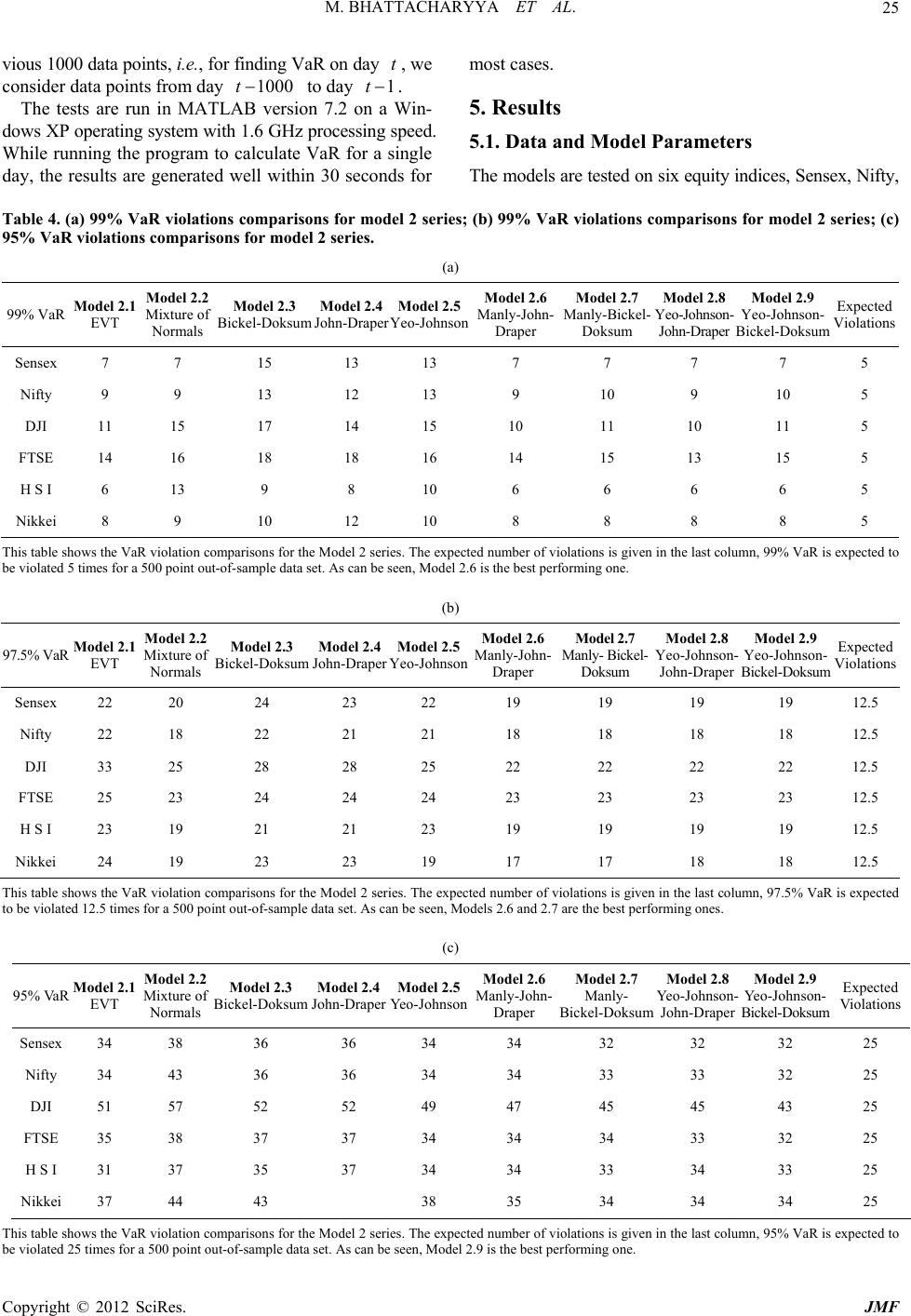

M. BHATTACHARYYA ET AL. 25
vious 1000 data points, i.e., for finding VaR on day t, we
consider data points from day t1000 to day 1t

.
re run in MATLAB version 7.2 on a Win-
ating system with 1.6 GHz processing speed.
hile running the program to calculate VaR for a single
Table 4. (a) 99% VaR violations comparisons for model 2 ser 99% VaR violations comparisons for model 2 series; (c)
95% VaR violations comparisons for model 2 series.
99% VaR odel 2.1
EVT
Model 2.2
Mixtur
Nors
Model 2.3
Bickel-Doksum
4
Draper
Model 2.5
Yeo-Johnson
Model 2.6
Manly-John-
Draper
Model 2.7
Manly-Bickel-
Doksum
Model 2.8
Yeo- ohnson-
John-Draper
Model 2.9
Yeo-Johnson-
Bickel-Doksu
Expected
Violations
The tests a
dows XP oper
W
day, the results are generated well within 30 seconds for The models are tested on six equity indices, Sensex, Nifty,
most cases.
5. Results
5.1. Data and Model Parameters
ies; (b)
(a)
Me of
mal John-
Model 2.J
m
Sensex 7 15 13 13 7 7 7 5 7 7
N9 13 12 9 10 9 10 5
D11 15 10 11 0 11 5
FT14 16 14 15 15 5
8 5
ifty 9 13
JI 15 17 14 1
SE 16 18 18 13
H S I 6 13 9 8 10 6 6 6 6 5
Nikkei 8 9 10 12 10 8 8 8
This table shows the VaR violation comparisons for the Model 2 series. The eted number of violations is given in the last column, 99% VaR is expected to
be violated 5 times for a 500 point out-of-sample data set. As can be seehe bene.
97.5% odel 2.1
EVT
Model 2.2
Mixtf
Normals
Model 2.3
Bickel-Doksu
odel 2.4
hn-Draper
Model 2.5
Yeo-Johnson
Model 2.6
Manly-John-
Draper
Model 2.7
anly- Bickel-
Doksum
Model 2.8
Yhnson-
John-Draper
Model 2.
Yeo-Johns
Bickel-Doksumiolations
xpec
n, Model 2.6 is t
(b)
st performing o
VaR Mure om
M
Jo Meo-Jo
9
on- Expected
V
Sensex 22 20 24 23 22 19 19 19 12.5 19
Nifty18 22 21 21 18 18 18 12.5
DJI 25 28 28 25 22 22 22 12.5
FTSE23 24 24 24 23 23 23 12.5
19 12.5
Nikkei 24 19 23 23 19 17 17 18 18 12.5
22 18
33 22
25 23
H S I 23 19 21 21 23 19 19 19
This table shows the VaR violation comparisons for the Model 2 serie numb is given in the last column, 97.5% VaR is expected
to be5 tim-of- As 2.6 aes
95% V aR odel 2.1
EVT
Mod2
Mixture of
Nor
Model 2.3
Bickel-Doksum
odel 2.4
hn-Draper
Model 2.5
Yeo-Johnson
Model 2.6
Manly-John-
Draper
Model 2.7
Manly-
ckel-Doksum
8
Yeo-Johnson-
Japer
Model 2.
Yeo-Johnson-
Bickel-Doks
Expected
Violations
s. The expected
can be seen, Models
er of violations
nd 2.7 are the b violated 12.es for a 500 point outsample data set.t performing ones.
(c)
Mel 2.
mals Jo
M
Bi
Model 2.
ohn-Dr
9
um
Sensex 34 38 36 36 32 32 25 34 34 32
Ni34 43 36 36 33 32 25
D51 57 52 52 45 43 25
8
fty 34 34 33
JI 49 47 45
FTSE 35 38 37 37 34 34 34 33 32 25
H S I 31 37 35 37 34
Nikkei 37 44 43 3
34 33 34 33 25
35 34 34 34 25
Thclations is given in the last column, 95% VaR is expected to
del 2.9 is the best performing one.
is table shows the VaR violation comparisons for the Model 2 series. The expeted number of vio
be violated 25 times for a 500 point out-of-sample data set. As can be seen, Mo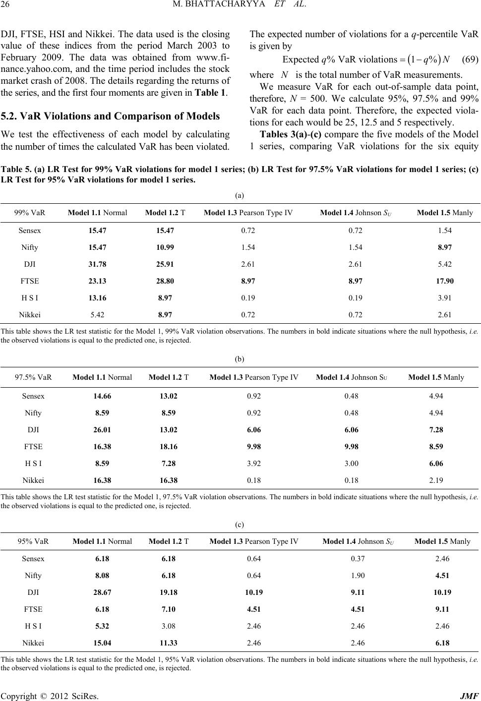

M. BHATTACHARYYA ET AL. 26
DJI, FTSE, HSI and Nikkei. The data used is the closing
d March 2003 to
ed from www.fi-
the series, and the first four moments are given in Table 1.
5.2. VaRne
We test thecti
ther othlculated VaR has bte
is given by
N (69)
We measure VaR for each out-of-sample data point,
therefore, N = 500. We calculate 95%, 97.5% and 99%
V che,ted viola-
tT 3(a)pa
1 ser, compariVaR vations fohe six eity
Table 5. (a) LR Test fo VaR violations for model 1 series; (b) LR Test for 97 VaR vioions for mel 1 series; (c)
LRt for VaR violations for model 1 series.
(a)
VaR Mode Normal 2 TMode Pearson T IV del 1.4 Johnson SU odel 1.5 Mly
value of these indices from the perio
ebruary 2009. The data was obtainF
nance.yahoo.com, and the time period includes the stock
market crash of 2008. The details regarding the returns of where N is the total number of VaR measurements.
Violations and Compariso
f each model
of Mod
by calcu
ls
lating effeveness o
e numbf times e caeen violad.
The expected number of violations for a q-percentile VaR

Expected % VaR violations1%qq
aR for ea
ions for eac
ables
data point
h would be 2
-(c) com
. Therefor
5, 12.5 and
re the five
the expec
5 respective
models of th
ly.
e Model
iesng iolr tqu
r 99%.5%latod
Tes95%
99% l 1.1 Model 1. l 1.3ype MoM an
Sensex 47 0.72 0.72 1.54 15.47 15.
Nifty 15.47 10.99 1.54 1.54 8.97
DJI 31.78 25.91 2.61 2.61 5.42
FTSE 23.13 28.80 8.97 17.90
H S .9
Nikkei 2
8.97
I 13.16 8
8.97
7 0.19 0.
0.7
19
0.72
3.
2.
91
61 5.42
Thow LR teststic for theel 1, 99% violation observations. bers in indicate sitns where tll hypot.
the observed violations is equal to the predicted one, is rejected.
(b)
VaRModel 1.1 Normal Mode l 1.2Model 1.3 Pearsope IV el 1.4 JohnU Model 1.5 M
his table ss the stati Mod VaRThe num bolduatiohe nuhesis, i.e
97.5% T n TyModson Sanly
Sensex .66 13.02 0.92 0.48 4.94 14
Nifty 59 8.59 0.92 0.48 4.94
8.59
H S I 8.59 7.28 92 3.00 6.06
16
8.
DJI 26.01 13.02 6.06 6.06 7.28
FTSE 16.38 18.16 9.98 9.98
3.
Nikkei 16.38 .38 0.18 0.18 2.19
This table showR tetiom
the observed violations is equal to the predicted one, is rejected.
(c)
Model 1.1 Normal Model 1.2 Model 1.3 Pearson Tpe IV 4 Johnson SU 5 Ma
s the Lst statistic for the Model 1, 97.5% VaR violation observans. The nubers in bold indicate situations where the null hypothesis, i.e.
95% VaR T yModel 1.Model 1.nly
Sensex 18 6.18 0.64 0.37 2.46 6.
Nifty 08 6.18 0.64 1.90 4.51
I .67 19.18 10.19 9.11 10.19
2.46 2.46
8.
DJ 28
FTSE 6.18 7.10 4.51 4.51 9.11
H S I 5.32 3.08 2.46
Nikkei 15.04 11.33 2.46 2.46 6.18
This table shows the LR test statistic for the Model 1, 95% VaR violation obsetions. The numbers in bold indicate situations where the null hypothesis, i.e.
the observed violations is equal to the predicted one, is rejected. rva

M. BHATTACHARYYA ET AL. 27
indices. Tables 4(a)-(c) compare the same for the nine
computed, and the best model for each percentile VaR is
found.
It can be seen that Models 1.3 and 1.4 are best per-
(where ARMA (1, 1)-GARCH (1, 1) pa-
rameters are calculated with the pseudo-normal a
wthe
Table 6. (a) LR Test for 99% VaR violations for model 2 series;
LR Test for 95% VaR violations for model 2 series.
(a)
Normals raper Yeo-Johnson Manly- John-Draper
Manly-Bickel-
Doksum
Yeo-Johnson-
John-Draper
Yeo-Johnson-
Bickel-Doksum
models of the Model 2 series. The expected violations for
99%, 97.5% and 95% VaR are given in the last column
of each table. The mean violation for each model is
forming models across all indices. Amongst those of the
Model 2 series
ssump-
tion) hoever, Models 2.6, 2.7, 2.8 and 2.9 perform
best. This is expected from the skewness-kurtosis Table
2, where the most normalized transformations are shown to
be Manly-John-Draper, Manly-Bickel-Doksum, Yeo-John-
(b) LR Test for 97.5% VaR violations for model 2 series; (c)
99% V aR Model 2.1
EVT
Model 2.2
Mixture of Model 2.3
Bickel-Doksum
Model 2.4
John-D
Model 2.5 Model 2.6 Model 2.7 Model 2.8 Model 2.9
Sensex 0.72 0.72 13.16 8.97 8.97 0.72 0.72 0.72 0.72
Nifty 2.61 2.61 8.97 7.11 8.97 2.61 3.91 2.61 3.91
DJI42 90 10.99 13.3.91 5.42 3.91
FTSE 10.99 15.20.46 20.46 15.10.99 13.16 8.97
H S I0.19 2.61 1.54 3.0.19 0.19 0.19
Nikkei 1.54 3.91 7.11 3.54 1.54 1.54
5.13.16 17.16 5.42
47 47 13.16
8.97 91 0.19
2.61 91 1.1.54
This tas the LR test sta for the Model 2, VaR violation obser The numbers in bold indications where the null hysis, i.e.
the obiolations is eque predicted one,cted.
aR Model 2. 1
EVT Mixture of
Normals
Model 2.3
Bickel-Doksum
Model 2.4
John-Draper
Model 2.5
Ye nson
Model 2.6
Manly-
John-Draper
Model 2.7
Manly-
Bickel-Doksum
Model 2.8
Yeo-Johnson-
John-Draper
Model 2.9
Yeo-Johnson-
Bickel-Doksum
ble showtistic 99%vations.te situapothe
served val to th is reje
(b)
Model 2.2
99% Vo-Joh
Se92 828 00 nsex 3.6.06 .59 7.6.06 3.00 3.00 3.3.00
Nif2.19 6.06 4.94 4.94 2.19 2.19 2.19 19
DJI 9.98 214.66 14.66 9.98 6.06 6.06 6.06 06
FTSE 7.28 8.59 8.59 8.59 7.28 7.28 7.28 28
H S3.00 4.94 4.94
7.2 3.00 3.00 3.00 00
Nikkei 3.00 7.28 7.28 3.00 1.50 1.50 2.19 19
ty 6.06 2.
3.95 6.
9.98 7.
I 7.28 8 3.
8.59 2.
This tas the LR test sr the Model 2,VaR violation obser The numbers in bold indtuations where the nuthesis, i.e.
(c)
99% VaR Model 2.1 Model 2.2 Mixture of Model 2.3
el-
Model 2.4
-Dra
Model 2.5 Model 2.6
Manly-
er
Model 2.7
Manly-Bickel-
Model 2.8
Yeo-Johnson-
aper
Model 2.9
Yeo-Johnson-
ble showtatistic fo 97.5% vations.icate sill hypo
the observed violations is equal to the predicted one, is rejected.
EVT Normals BickDoksum JohnperYeo-Johnson John-Drap Doksum John-Dr Bickel-Doksum
Sensex 3.08 64.51 4.51 3.08 3.08 1.90 1.90
.18 1.90
Nif3.08 14.51 4.51 3.08 3.08 2.46 2.46
DJI 22.17 323.7323.73 19.16.37 13.75 13.75
FTS3.77 65.32 5.32 3.08 3.08 3.08 2.46
H S1.41 53.77 5.32 3.08 3.08 2.46 3.08
Nik 5.32 111.3311.33 6.18 3.77 3.08 3.08
ty 1.33 1.90
2.16 18 11.33
E .18 1.90
I .32 2.46
kei 2.52 3.08
This table shows the LR test statistic for the Model 2, 95% VaR violation observations. The numbers in bold indicate situations where the null hypothesis, i.e.
e observed violations is equal to the predicted one, is rejected. th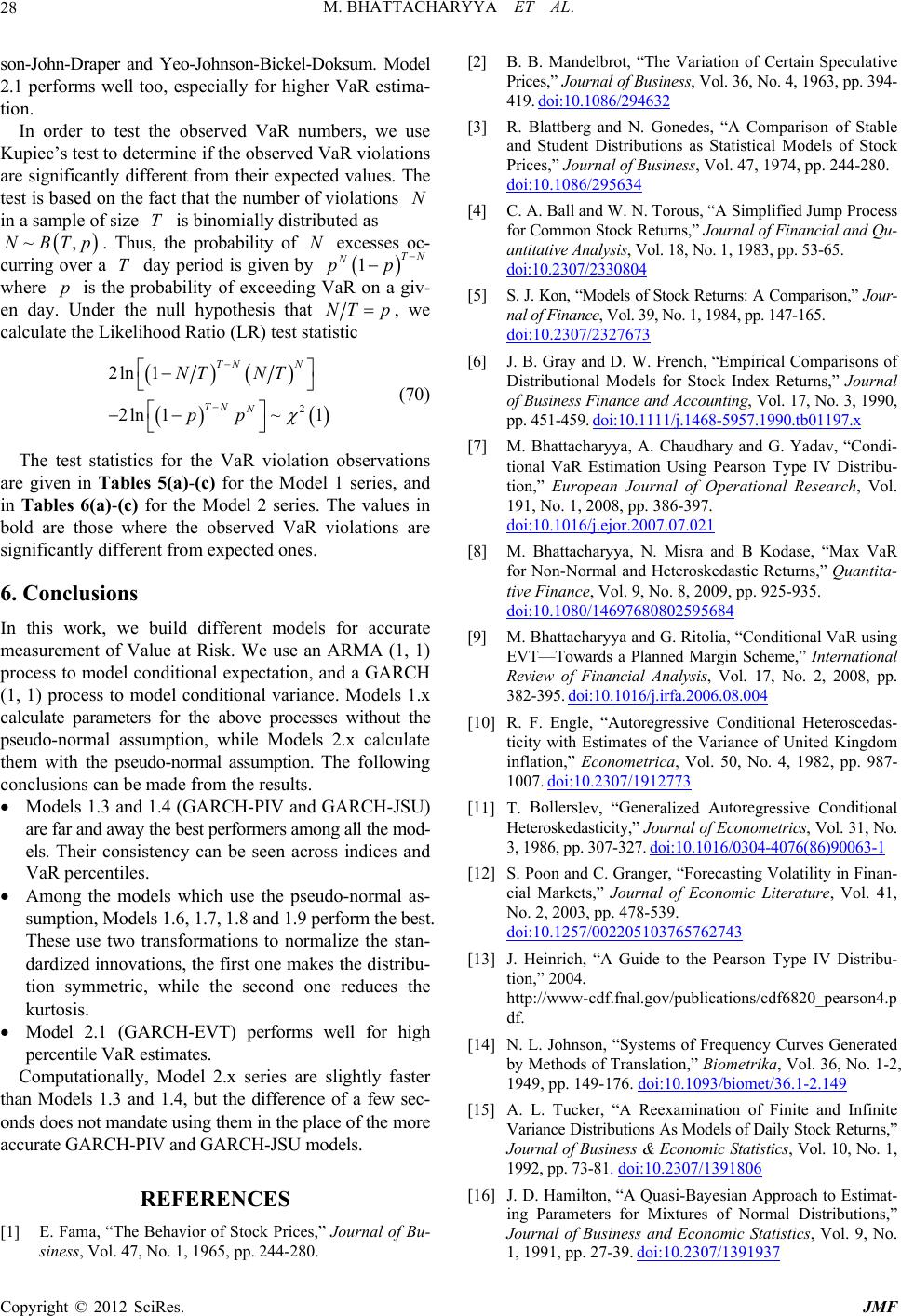

M. BHATTACHARYYA ET AL. 28
son-John-Draper and Yeo-Johnson-Bickel-Doksum. Model
2.1 performs well too, especially for higher VaR estima-
tion.
In order to test the observed VaR numbers, we use
Kupiec’s test to determine if the observed VaR violations
are significantly different from their expected values. The
test is based on the fact that the number of violations N
in a sample of size T is binomially distributed as

~,Tp. Thus, the probability of N excesses oc- NB
curring over a T day period is given by

1TN
N
pp


where p is the probability of exceeding VaR on a giv-
en day. Under the null hypothesis that NT p

, we
calculate the Likelih (LR) test statood Ratioistic

N N
NT

 
1
ln 11
N
p




(70)
Thstatistics foVaR v observtions
areen inles 5 for tdel 1 , and
in s 6) forodel s. Thes in
bo thohereobserveR viols are
signintlyrent fr expected es.
measurement of Value at Risk. We use an ARMA (1, 1)
process to mexpd a GARCH
o
calculate parters th
pormssump while Models 2.x calculate
theith thal assumThe fwing
coionsadm the rs.
 dels 1.3 and 1.4-Pd GARSU)
r and away the performmong almod-
r consistency can be seen across in
peres.
ng odelsh use tseudo-nl as-
dardized innovations, the first one makes the distribu-
tion symmetric, while the second one reduces the
kurtosi

percentile VaR es
utatly, M 2.x sere slighaster
thsand 1t the dince of a few sec-
onds does notndatethem imore
accurate GARCH-PIV and GARCH-JSU model
RE NC
[1 ame Behavior of Stock Prices,” Journal of Bu-
siness, Vol. 47, No. 1, 1965, pp. 244-280.
[2] B. B. Mandelbrot, “The Variation of Certain Speculative
2
~ 

2ln
2
T
NT

TN
p 

e test
giv
r the
(a)-(c) iolation he Mo
a
series Tab
Table (a)-(c the M2 seriee valu
ld are
fica
se w
diffe
the
om
d Va
on
ation
6. Conclusions
this work, we build different models for accurateIn
odel co
ces m
nditional ectation, an
ional variance
cesses w
(1, 1) pros to
ame
del condit
for the above pro
. Models 1
ithout
.x
e
seudo-nal ation,
m w
nclus
e pseudo-nor
can be m
m
e fro
ption.
esult
ollo
Mo (GARCHIV anCH-J
are fa
els. Thei
best ers al the
dices and
VaR centil
Amothe m whiche porma
sumption, Models 1.6, 1.7, 1.8 and 1.9 perform the best.
These use two transformations to normalize the stan-
s.
2 A Model.1 (GRCH-EVT
timates.
) performs well for high
Compionalodelries atly f
an Model 1.3
ma
.4, bu
using
ffere
n the place of the
s.
FEREES
] E. Fa, “Th
Prices,” Journal of Business, Vol. 36, No. 4, 1963, pp. 394-
419. doi:10.1086/294632
[3] R. Blattberg and N. Gonedes, “A Comparison of Stable
and Student Distributions as Statistical Models of Stock
Prices,” Journal of Business, Vol. 47, 1974, pp. 244-280.
doi:10.1086/295634
[4] C. A. Ball and W. N. Torous, “A Simplified Jump Process
for Common Stock Returns,” Journal of Financial and Qu-
antitative Analysis, Vol. 18, No. 1, 1983, pp. 53-65.
doi:10.2307/2330804
[5] S. J. Kon, “Models of Stock Returns: A Comparison,” Jour-
nal of Finance, Vol. 39, No. 1, 1984, pp. 147-165.
/23doi:10.2307 27673
d D. W. Frenc
odels fo
[6] J. anhf
al Mr St
of Bss Finance and Accountol. 17, N990,
pp. 59. doi:1 1/j.1468-5 990.tb011
B. Gray
Distribution
, “Empirical C
ock Index Re
omparisons o
turns,” Journal
usine
451-4
ing, V
957.1
o. 3, 1
97.x0.111
[7] M. Bhattacharyya, A. Chaudharyav ndi-
tional VaR Estimation Using Pearson Type IV Distribu-
tion,” Journal of Operational Reseaol.
191, No. 1, 20086-397.
doi:10.1016/j.ejor.2007.07.021
and G. Yad, “Co
European rch, V
, pp. 38
[8] M. Bhattacharyya, N. Misra and B Kodase, “Max VaR
for Non-Normal and Heteroskedeturns,” tita-astic RQuan
tive Finance, Vol. 9, No. 8, 2009, pp. 925-935.
doi:10.1080/14697680802595684
[9] M. Bhattacharyya and G. Ritolia, “Conditional VaR using
EVT—Towards a Planned Margin Scheme,” International
Finlysi No.p.
30.fa.2
Review of
82-395.
ancial Ana
1016/j.ir
s, Vol. 17,
006.08.004
2, 2008, p
doi:1
[10] a -
ticth Estimates of the Variance of United Kingdom
inflat” Econometrica, Vol. 5. 4, 1982,
10 i:10.230 2773
R. F. Engle, “Autoregressive Condition l Heteroscedas
ity wi
ion,
07.
0, Nopp. 987-
do7/191
1] T. lev, “alized Agressive Cional
Heteroskedasticit urnal of Econometrics, V, No.
3, 1986, pp. 307-oi:10.101 4-4076(863-1
[1 BollersGenerutoreondit
y,” Jo
327.
ol. 31
)9006d 6/030
2] S. Poon and C. Granger, “Forecasting Volatilitinan-
ciaets,” Journal of Econ Literaturl. 41,
No. 2, 2003, pp. 478-539.
[1 y in F
l Markomic e, Vo
doi:10.1257/002205103765762743
[13] J. Heinrich, “A Guide to the Pearson Type IV Distribu-
tion,” 2004.
http://www-cdf.f publications/cdf6820_pearson4.p
on,s of
by Methods of Translation,” Bioika, Vol. 36. 1-2,
nal.gov/
“System
df.
N. L. Johns[14] Frequency Curves Generated
metr , No
1949, pp. 149-17:10.1093et/36.1-2.6. doi /biom149
[15] A.ucker, “examinatf Finite afinite
Variance Distribdaily Stock Returns,”
Journal of Businomstics, Vol. 10, No. 1,
L. TA Reion ond In
utions As Mo
ess & Econ
els of D
ic Stati
19. 73-81. /1392, ppdoi:10.2307 91806
6] J. D. Hamilton, “asi-Bayepproach imat-
ing Parameters for Mixtures of
Journal of Busind Econotatistics, , No.
1, 1991, pp. 27-39. doi:10.2307/1391937
[1 A Qusian A
Normal Distributions,”
to Est
ess anmic SVol. 9

M. BHATTACHARYYA ET AL. 29
[17] D. M. Titterington, A. F. M Smitha and U. E. Makov,
“Statistical Analysis of Finite Mixture Distributions,” John
Variables Are Not Normally Distributed,”
Wiley & Sons, Chichester, 1992.
[18] J. Hull and A. White, “Value at Risk When Daily Changes
in Market Jour-
nal of Derivatives, Vol. 5, No. 3, 1998, pp. 9-19.
doi:10.3905/jod.1998.4 07998
[19] P. Zangari, “An Improved Methodology for Measuring
VaR,” Risk Metrics Monitor, Reuters/JP Morgan, 1996.
[20] G. E. P. Box an D. R. Cox, “An Analysis of Tra
” Journal of the Royal StatisticaSociety, Vol. 26,
No. 2, 1964, pp. 211-252.
[21] B. F. J. Manly, “Exponential Data Transformations,” The
Statistician, Vol. 25, No. 1, 1976, pp. 37-4
d nsfor-
mations, l
2.
doi:10.2307/2988129
[22] P. Li, “Box Cox Transformations: An Overview,” Uni-
versity of Connecticut, Storrs, 2005.
[23] P. J. Bickel and K. A. Doksum, “An Ana
Association, Vol. 76, 1981, pp. 296-311.
lysis of Trans-
formations Revisited,” Journal of the American Statistical
doi:10.2307/2287831
[24] J. A. John and N. R. Draper, “An Alternative Family of
Transformations,” Applied Statistics, Vol. 29, No. 2, 1980,
pp. 190-197. doi:10.2307/2986305
[25] I.-K. Yeo and R. Johnson, “A New Family of Power Trans-
formations to Improve Normality or Symmetry,” Biome-
trika, Vol. 87, No. 4, 2000, pp. 954-959.
doi:10.1093/biomet/87.4.954
[26] W. K. Newey and D. G. Steigerwald, “Asymptotic Bias
for Quasi-Maximum-Likelihood Estimators in Condi-
tional Heteroskedasticity Models,” Econometrica, Vol. 65,
No. 3, 1997, pp. 587-599. doi:10.2307/2171754
[27] P. G. Perez, “Capturing Fat Tail Risk in Exchange Rate
l of Risk,
008, pp. 73-100.
Returns Using SU-Curves: A Comparison with Normal Mix-
ture and Skewed Student Distributions,” Journa
Vol. 10, No. 2, 2007-2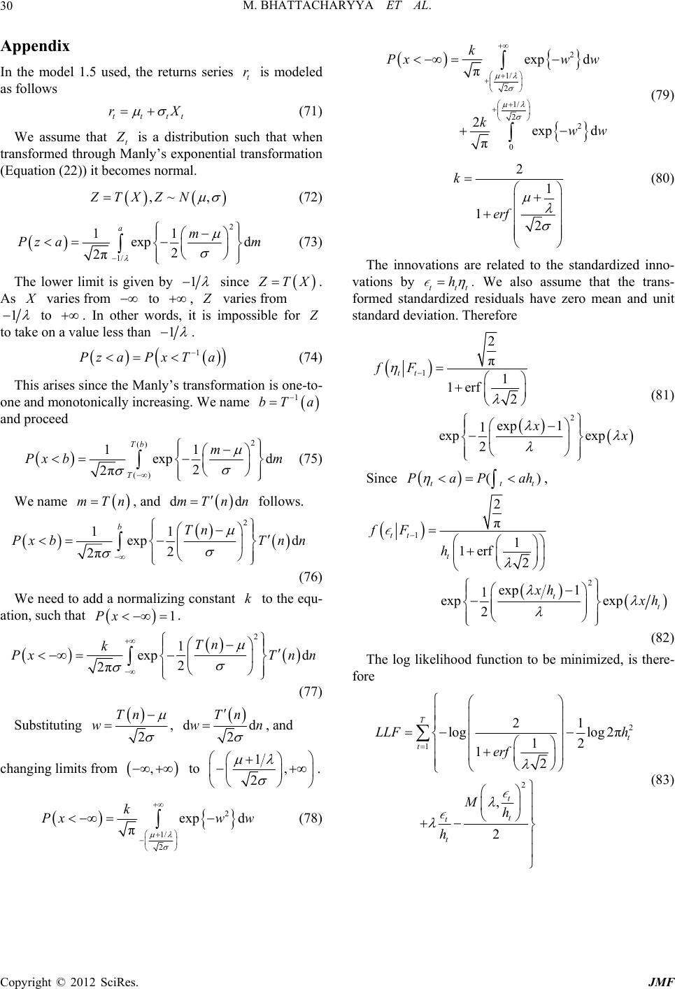

M. BHATTACHARYYA ET AL. 30
Appendix
In the model 1.5 used, the returns series t r is modeled
as follows
tttt
rX

  (71)
We assume that t
Z
is a distribution such that when
transformed through Manly’s exponential transformation
(Equation (22)) it becomes normal.
 
,~ZTXZN,

  (72)

2
11
1/ 2
2exp d
am
z am



 
  (73
π
P








)
The lower limit is given b y 1

 since


Z
TX.
As
X
varies from  to

,
Z
varies from
1

 to  . In other words, it is impossible for
Z
to take on a value less than 1

.
 

1
PzaPxTa

  (74)
This arises since the Manly’s transformation is one-to-
one and monotonically increasing. We name


1
bTa


and proceed

2
()
()
11
exp d
2
2π
Tb
T
m
Px bm








 








 (75)
We name , and follows.

mTn

ddmTnn


  
2
11
exp d
2
2π
bTn
PxbT nn











 


(76)
We need to add a normalizing constant to the equ-
ation, such that
k

1Px .
  
2
1
exp d
2
2π
Tn
k
PxT nn









 





(77)
Substituting

2
Tn
w



,

dd
2
Tn
wn


, and
changing limits from to

,1,
2


 






.



2
1/
2
exp d
π
k
Pxw w



 


 



(78)

2
1/
2
1/
exp d
π
Pxw w



 





 

2
2
0
2
expd
π
kww




k

(79)
2
1
1
k
2
erf







(80)



The innovations are related to the standardized inno-
vations by ttt h


 . We also assume that the trans-
formed standardized residuals have zero mean and unit
standard deviation. Therefore

 
1
2
2
π
1
1erf2
exp 1
1
expexp
2
tt
fF
x



x














(81)
Since


()
tt
PaPah   
, t

 
1
2
2
π
1
1erf 2
exp 1
1
expexp
2
tt
t
t
t
fF
h
xh
x
h











 




 


(82)
The log likelihood function to be minimized, is there-
fore
2
1
2
21
loglog 2π
2 1
12
,
2
T
t
t
t
t
t
t
LLF h
erf
Mh
h







 














 






(83)