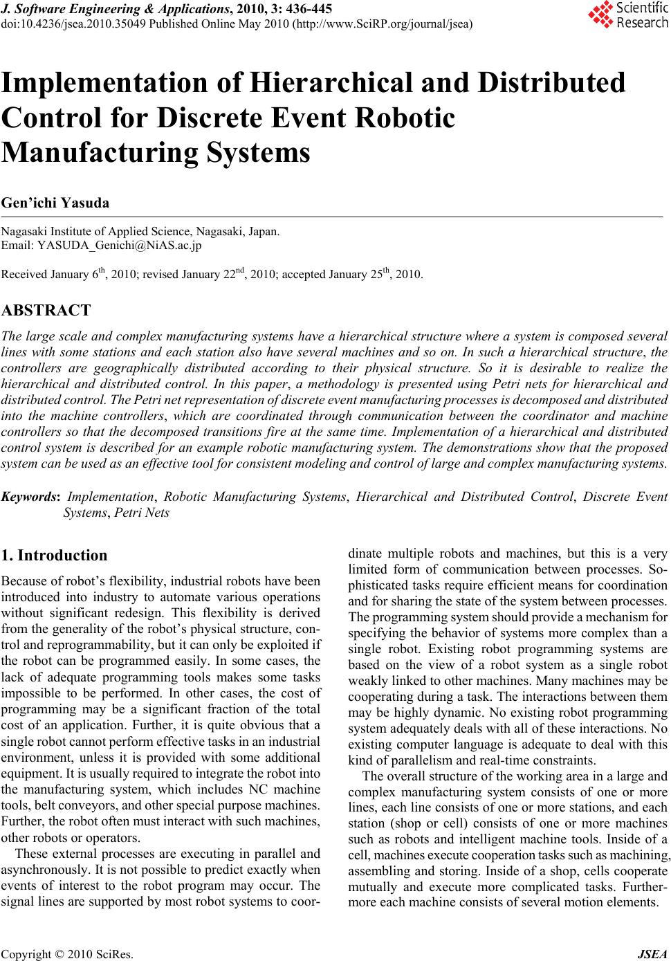J. Software Engineering & Applications, 2010, 3: 436-445
doi:10.4236/jsea.2010.35049 Published Online May 2010 (http://www.SciRP.org/journal/jsea)
Implementation of Hierarchical and Distributed
Control for Discrete Event Robotic
Manufacturing Systems
Gen’ichi Yasuda
Nagasaki Institute of Applied Science, Nagasaki, Japan.
Received January 6th, 2010; revised January 22nd, 2010; accepted January 25th, 2010.
ABSTRACT
The large scale and complex manufacturing systems have a hierarchical structure where a system is composed several
lines with some stations and each station also have several machines and so on. In such a hierarchical structure, the
controllers are geographically distributed according to their physical structure. So it is desirable to realize the
hierarchical and distributed control. In this paper, a methodology is presented using Petri nets for hierarchical and
distributed control. The Petri net representation of discrete event manufacturing processes is decomposed and distributed
into the machine controllers, which are coordinated through communication between the coordinator and machine
controllers so that the decomposed transitions fire at the same time. Implementation of a hierarchical and distributed
control system is described for an example robotic manufacturing system. The demonstrations show that the proposed
system can be used as an effective tool for consistent modeling and control of large and complex manufacturing systems.
Keywords: Implementation, Robotic Manufacturing Systems, Hierarchical and Distributed Control, Discrete Event
Systems, Petri Nets
1. Introduction
Because of robot’s flexibility, industrial robots have been
introduced into industry to automate various operations
without significant redesign. This flexibility is derived
from the generality of the robot’s physical structure, con-
trol and reprogrammability, but it can only be exploited if
the robot can be programmed easily. In some cases, the
lack of adequate programming tools makes some tasks
impossible to be performed. In other cases, the cost of
programming may be a significant fraction of the total
cost of an application. Further, it is quite obvious that a
single robot cannot perform effective tasks in an industrial
environment, unless it is provided with some additional
equipment. It is usually required to integrate the robot into
the manufacturing system, which includes NC machine
tools, belt conveyors, and other special purpose machines.
Further, the robot often must interact with such machines,
other robots or operators.
These external processes are executing in parallel and
asynchronously. It is not possible to predict exactly when
events of interest to the robot program may occur. The
signal lines are supported by most robot systems to coor-
dinate multiple robots and machines, but this is a very
limited form of communication between processes. So-
phisticated tasks require efficient means for coordination
and for sharing the state of the system between processes.
The programming system should provide a mechanism for
specifying the behavior of systems more complex than a
single robot. Existing robot programming systems are
based on the view of a robot system as a single robot
weakly linked to other machines. Many machines may be
cooperating during a task. The interactions between them
may be highly dynamic. No existing robot programming
system adequately deals with all of these interactions. No
existing computer language is adequate to deal with this
kind of parallelism and real-time constraints.
The overall structure of the working area in a large and
complex manufacturing system consists of one or more
lines, each line consists of one or more stations, and each
station (shop or cell) consists of one or more machines
such as robots and intelligent machine tools. Inside of a
cell, machines execute cooperation tasks such as machining,
assembling and storing. Inside of a shop, cells cooperate
mutually and execute more complicated tasks. Further-
more each machine consists of several motion elements.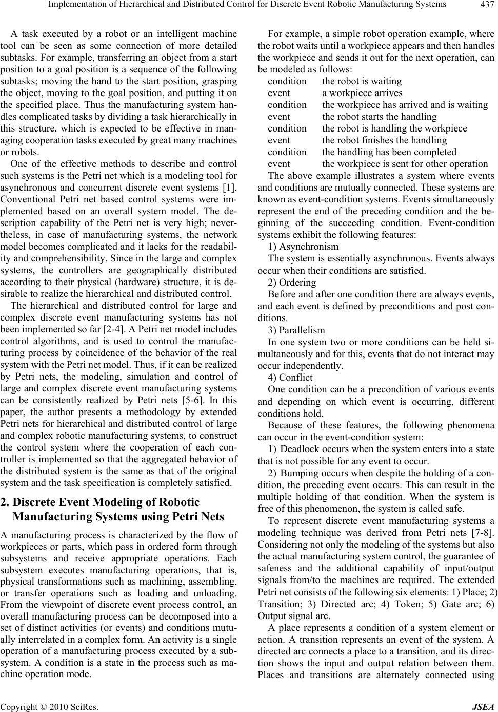

Implementation of Hierarchical and Distributed Control for Discrete Event Robotic Manufacturing Systems 437
A task executed by a robot or an intelligent machine
tool can be seen as some connection of more detailed
subtasks. For example, transferring an object from a start
position to a goal position is a sequence of the following
subtasks; moving the hand to the start position, grasping
the object, moving to the goal position, and putting it on
the specified place. Thus the manufacturing system han-
dles complicated tasks by dividing a task hierarchically in
this structure, which is expected to be effective in man-
aging cooperation tasks executed by great many machines
or robots.
One of the effective methods to describe and control
such systems is the Petri net which is a modeling tool for
asynchronous and concurrent discrete event systems [1].
Conventional Petri net based control systems were im-
plemented based on an overall system model. The de-
scription capability of the Petri net is very high; never-
theless, in case of manufacturing systems, the network
model becomes complicated and it lacks for the readabil-
ity and comprehensibility. Since in the large and complex
systems, the controllers are geographically distributed
according to their physical (hardware) structure, it is de-
sirable to realize the hierarchical and distributed control.
The hierarchical and distributed control for large and
complex discrete event manufacturing systems has not
been implemented so far [2-4]. A Petri net model includes
control algorithms, and is used to control the manufac-
turing process by coincidence of the behavior of the real
system with the Petri net model. Thus, if it can be realized
by Petri nets, the modeling, simulation and control of
large and complex discrete event manufacturing systems
can be consistently realized by Petri nets [5-6]. In this
paper, the author presents a methodology by extended
Petri nets for hierarchical and distributed control of large
and complex robotic manufacturing systems, to construct
the control system where the cooperation of each con-
troller is implemented so that the aggregated behavior of
the distributed system is the same as that of the original
system and the task specification is completely satisfied.
2. Discrete Event Modeling of Robotic
Manufacturing Systems using Petri Nets
A manufacturing process is characterized by the flow of
workpieces or parts, which pass in ordered form through
subsystems and receive appropriate operations. Each
subsystem executes manufacturing operations, that is,
physical transformations such as machining, assembling,
or transfer operations such as loading and unloading.
From the viewpoint of discrete event process control, an
overall manufacturing process can be decomposed into a
set of distinct activities (or events) and conditions mutu-
ally interrelated in a complex form. An activity is a single
operation of a manufacturing process executed by a sub-
system. A condition is a state in the process such as ma-
chine operation mode.
For example, a simple robot operation example, where
the robot waits until a workpiece appears and then handles
the workpiece and sends it out for the next operation, can
be modeled as follows:
condition the robot is waiting
event a workpiece arrives
condition the workpiece has arrived and is waiting
event the robot starts the handling
condition the robot is handling the workpiece
event the robot finishes the handling
condition the handling has been completed
event the workpiece is sent for other operation
The above example illustrates a system where events
and conditions are mutually connected. These systems are
known as event-condition systems. Events simultaneously
represent the end of the preceding condition and the be-
ginning of the succeeding condition. Event-condition
systems exhibit the following features:
1) Asynchronism
The system is essentially asynchronous. Events always
occur when their conditions are satisfied.
2) Ordering
Before and after one condition there are always events,
and each event is defined by preconditions and post con-
ditions.
3) Parallelism
In one system two or more conditions can be held si-
multaneously and for this, events that do not interact may
occur independently.
4) Conflict
One condition can be a precondition of various events
and depending on which event is occurring, different
conditions hold.
Because of these features, the following phenomena
can occur in the event-condition system:
1) Deadlock occurs when the system enters into a state
that is not possible for any event to occur.
2) Bumping occurs when despite the holding of a con-
dition, the preceding event occurs. This can result in the
multiple holding of that condition. When the system is
free of this phenomenon, the system is called safe.
To represent discrete event manufacturing systems a
modeling technique was derived from Petri nets [7-8].
Considering not only the modeling of the systems but also
the actual manufacturing system control, the guarantee of
safeness and the additional capability of input/output
signals from/to the machines are required. The extended
Petri net consists of the following six elements: 1) Place; 2)
Transition; 3) Directed arc; 4) Token; 5) Gate arc; 6)
Output signal arc.
A place represents a condition of a system element or
action. A transition represents an event of the system. A
directed arc connects a place to a transition, and its direc-
tion shows the input and output relation between them.
Places and transitions are alternately connected using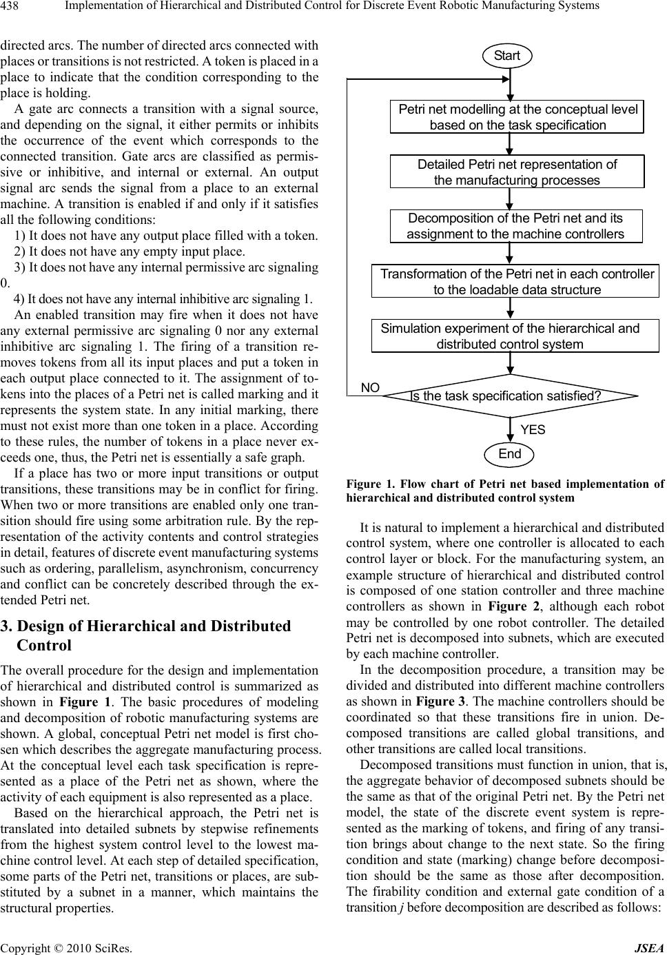

Implementation of Hierarchical and Distributed Control for Discrete Event Robotic Manufacturing Systems 438
directed arcs. The number of directed arcs connected with
places or transitions is not restricted. A token is placed in a
place to indicate that the condition corresponding to the
place is holding.
A gate arc connects a transition with a signal source,
and depending on the signal, it either permits or inhibits
the occurrence of the event which corresponds to the
connected transition. Gate arcs are classified as permis-
sive or inhibitive, and internal or external. An output
signal arc sends the signal from a place to an external
machine. A transition is enabled if and only if it satisfies
all the following conditions:
1) It does not have any output place filled with a token.
2) It does not have any empty input place.
3) It does not have any internal permissive arc signaling
0.
4) It does not have any internal inhibitive arc signaling 1.
An enabled transition may fire when it does not have
any external permissive arc signaling 0 nor any external
inhibitive arc signaling 1. The firing of a transition re-
moves tokens from all its input places and put a token in
each output place connected to it. The assignment of to-
kens into the places of a Petri net is called marking and it
represents the system state. In any initial marking, there
must not exist more than one token in a place. According
to these rules, the number of tokens in a place never ex-
ceeds one, thus, the Petri net is essentially a safe graph.
If a place has two or more input transitions or output
transitions, these transitions may be in conflict for firing.
When two or more transitions are enabled only one tran-
sition should fire using some arbitration rule. By the rep-
resentation of the activity contents and control strategies
in detail, features of discrete event manufacturing systems
such as ordering, parallelism, asynchronism, concurrency
and conflict can be concretely described through the ex-
tended Petri net.
3. Design of Hierarchical and Distributed
Control
The overall procedure for the design and implementation
of hierarchical and distributed control is summarized as
shown in Figure 1. The basic procedures of modeling
and decomposition of robotic manufacturing systems are
shown. A global, conceptual Petri net model is first cho-
sen which describes the aggregate manufacturing process.
At the conceptual level each task specification is repre-
sented as a place of the Petri net as shown, where the
activity of each equipment is also represented as a place.
Based on the hierarchical approach, the Petri net is
translated into detailed subnets by stepwise refinements
from the highest system control level to the lowest ma-
chine control level. At each step of detailed specification,
some parts of the Petri net, transitions or places, are sub-
stituted by a subnet in a manner, which maintains the
structural properties.
Start
Petri net modelling at the conceptual level
based on the task specification
Detailed Petri net representation of
the manufacturing processes
Decomposition of the Petri net and its
assignment to the machine controllers
Transformation of the Petri net in each controller
to the loadable data structure
Simulation experiment of the hierarchical and
distributed control system
Is the task specification satisfied?
End
YES
NO
Figure 1. Flow chart of Petri net based implementation of
hierarchical and distributed control system
It is natural to implement a hierarchical and distributed
control system, where one controller is allocated to each
control layer or block. For the manufacturing system, an
example structure of hierarchical and distributed control
is composed of one station controller and three machine
controllers as shown in Figure 2, although each robot
may be controlled by one robot controller. The detailed
Petri net is decomposed into subnets, which are executed
by each machine controller.
In the decomposition procedure, a transition may be
divided and distributed into different machine controllers
as shown in Figure 3. The machine controllers should be
coordinated so that these transitions fire in union. De-
composed transitions are called global transitions, and
other transitions are called local transitions.
Decomposed transitions must function in union, that is,
the aggregate behavior of decomposed subnets should be
the same as that of the original Petri net. By the Petri net
model, the state of the discrete event system is repre-
sented as the marking of tokens, and firing of any transi-
tion brings about change to the next state. So the firing
condition and state (marking) change before decomposi-
tion should be the same as those after decomposition.
The firability condition and external gate condition of a
transition j before decomposition are described as follows:

Implementation of Hierarchical and Distributed Control for Discrete Event Robotic Manufacturing Systems 439


R
r
II
rj
Q
q
IP
qj
N
n
O
nj
M
m
I
mjj
kgkg
kpkpkt
1
,
1
,
1
,
1
,
)()(
)()()(




(1)

V
v
EI
vj
U
u
EP
uj
E
jkgkgkg
1
,
1
,)()()(

 (2)
where,
M
: input place set of transition
j
;
)(
,kpI
mj : state of input placemof transitionj at time
sequence k;
N: output place set of transitionj;
)(
,kpO
nj : state of output placenof transition
j
at time
sequence k;
Q: internal permissive gate signal set of transition
j
;
)(
,kg IP qj : internal permissive gate signal variableqof
transition j at time sequence k;
R
: internal inhibitive gate signal set of transitionj;
)(
,kg II
rj : internal inhibitive gate signal variable
r
of
transition
j
at time sequence k;
U: external permissive gate signal set of transition
j
;
)(
,kg EP
uj : external permissive gate signal variable u
of transition
j
at time sequence k;
V: external inhibitive gate signal set of transition
j
;
Station controller
Robot
controller
MC
controller
Conveyor
controller
Machining
Center1 Conveyor2
Robot Machining
Center2
Conveyor1
Figure 2. Example structure of distributed control system
t1 t2
t11 t21 t12 t22t3 t4
decomposition
Station
controller
Machine
controller
t11,t21,t12,t22: global transition
t3,t4: local transition
Figure 3. Decomposition of transition
)(
,kg EI vj : external inhibitive gate signal variablevof
transition jat time sequence k;
The state (marking) change, that is, the addition or
removal of a token of a place, is described as follows:
))()(()()1( ,, kgktkpkpE
jj
I
mj
I
mj  (3)
))()(()()1(,, kgktkpkp E
jj
O
nj
O
nj  (4)
If transition
j
is divided into
s
transitions 1j,2j, , ,s
j
,
the firability condition of a transition after decomposition
is described as follows:


Rsub
r
II
rjsub
Qsub
q
IP
qjsub
Nsub
n
O
njsub
Msub
m
I
mjsubjsub
kgkg
kpkpkt
1
,
1
,
1
,
1
,
)()(
)()()(




(5)

Vsub
v
EI
vjsub
Usub
u
EP
ujsub
E
jsub kgkgkg
1
,
1
,)()()(

 (6)
From Equation (1) and Equation (5),

S
sub
jsubjktkt
1
)()(

 (7)
From Equation (2) and Equation (6),
)()(
1
kgkg
S
sub
E
jsub
E
j

 (8)
where,
S: total number of subnets
Msub : input place set of transitionjsub of subnet
sub ;
)(
,kpI
mjsub : state of input placemof transitionjsubof
subnet sub at time sequence k;
Nsub : output place set of transitionjsub of subnet
sub ;
)(
,kpO
njsub : state of output placenof transitionjsub of
subnet subat time sequence k;
Qsub : internal permissive gate signal set of transi-
tion jsub of subnetsub ;
Rsub : internal inhibitive gate signal set of transi-
tion jsub of subnet sub ;
Usub : external permissive gate signal set of transi-
tion jsub of subnet sub ;
Vsub : external permissive gate signal set of transi-
tion jsub of subnet sub ;

Implementation of Hierarchical and Distributed Control for Discrete Event Robotic Manufacturing Systems 440
The addition or removal of a token of a place con-
nected to a decomposed transition is described as fol-
lows:
))()(()()1( ,, kgktkpkp E
jj
I
mjsub
I
mjsub  (9)
))()(()()1( ,, kgktkpkp E
jj
O
njsub
O
njsub  (10)
Consequently it is proved that the firability condition
of the original transition is equal to AND operation of
firability conditions of decomposed transitions. If and
only if all of the decomposed transitions are enabled,
then the global transitions are enabled. To exploit the
above results, the coordinator program has been intro-
duced to coordinate the decomposed subnets so that the
aggregate behavior of decomposed subnets is the same as
that of the original Petri net.
There may exist a place which has plural input transi-
tions and/or plural output transitions. This place is called
a conflict place. The transitions connected to a conflict
place are in conflict when some of them are enabled at
the same time. In this case, only one of them fires and the
others become disabled. The choice for firing is done
arbitrarily using an arbiter program.
In case that a transition in conflict with other transi-
tions is decomposed as shown in Figure 4, these transi-
tions should be coordinated by the station controller. If
arbitration of the transitions is performed independently
in separate subnets, the results may be inconsistent with
the original rule of arbitration. Therefore the transitions
should be arbitrated together as a group. On the other
hand, arbitration of local transitions in conflict is per-
formed by local machine controllers.
The Petri net based control structure with introduction
of coordinator is shown in Figure 5. The control soft-
ware is distributed into the station controller and machine
controllers. The station controller is composed of the
Petri net based controller and the coordinator. The con-
ceptual Petri net model is allocated to the Petri net based
controller for management of the overall system. For
cooperative or exclusive tasks between robots, global
transitions at the station controller are used to communi-
cate the status of the robots. The detailed Petri net mod-
els are allocated to the Petri net based controllers in the
machine controllers. Each machine controller directly
monitors and controls the sensors and actuators of its
machine.
The control of the overall system is achieved by coor-
dinating these Petri net based controllers. System coor-
dination is performed through communication between
the coordinator in the station controller and the Petri net
based controllers in the machine controllers as the fol-
lowing steps.
1) When each machine controller receives the start
signal from the coordinator, it tests the firability of all
decomposition
t1
t2
t3
t1
t21
t22
t3
t21,t22: global transition
t1,t3: local transition
Figure 4. Decomposition of transition in conflict
Station
controller
Mac hi ne
controller
Global model
Machine 1 model
Machine 1 Machine N
Machine N model
Coordinator
Petri net engine
Petri net engine Petri net engine
Firability test result of
global transitions in
machine 1 model
Determination of firing
global transitions
Firability test result of
global transitions in
machine N model
Figure 5. Petri net based control structure with coordinator
transitions in its own Petri net, and sends the information
on the global transitions and the end signal to the coor-
dinator.
2) The coordinator tests the firability of the global
transitions, arbitrates conflicts among global and local
transitions, and sends the names of firing global transi-
tions and the end signal to the machine controllers.
3) Each machine controller arbitrates conflicts among
local transitions using the information from the coordi-
nator, generates a new marking, and sends the end signal
to the coordinator.
4) When the coordinator receives the end signal from
all the machine controllers, it sends the output command
to the machine controllers.
5) Each machine controller outputs the control signals
to its actuators.
Multilevel hierarchical and distributed control for
large and complex manufacturing systems can be con-
structed such that the control system structure corre-
sponds to the hierarchical and distributed structure of the
general manufacturing system. The coordination mecha-

Implementation of Hierarchical and Distributed Control for Discrete Event Robotic Manufacturing Systems 441
nism is implemented in each layer repeatedly as shown in
Figure 6. The overall system is consistently controlled,
such that a coordinator in a layer coordinates one-level
lower Petri net based controllers and is coordinated by
the one-level upper coordinator.
The details of coordination in a two-level control sys-
tem composed of a global controller and several local
controllers have been implemented as shown in Figure 7.
4. Implementation of Control System
4.1 Example of Workstation Task
The basic procedures of modeling and decomposition of
robotic manufacturing systems are shown through a sim-
ple example. The example robotic manufacturing system
is composed of two input conveyors, two machining
centers, one handling robot, and one output conveyor as
shown in Figure 8.
System
controller
Line
controller
Station
controller
Machine
controll e r
: Coordinator
: Petri net based controller
Figure 6. Hierarchical and distributed control structure for
overall manufacturing system
Holding of external gates
Firability test of all transitions
Firability test of global transitions
Arbitration of conflicts concerning global transitions
Determination of firing global transitions
Arbitration of conflicts among local transitions
Generation of a new marking
Reception of end signal from its local controllers
Output of control signals to its actuators
Start
Local coordinator Petri net based
controller
from
coordinator
to coordinator
Holding of external gate
s
Firability test of all transition
s
Firability test of global transitions
Arbitration of conflicts concerning global transitions
Determination of firing global transitions
Arbitration of conflicts among local transition
s
Generation of a new marking
Reception of end signal from the global controller
and all local coordinators
End
Sta r t
Global coordinator Petri net based
controller
to subsystems
from
subsystems
Figure 7. Flowchart of coordination in two-level control system

Implementation of Hierarchical and Distributed Control for Discrete Event Robotic Manufacturing Systems 442
CV2 CV1
MC1 MC2
CV3
Robot
A B
A B
A
B
A B B
Figure 8. Example of robotic manufacturing system
The task specification of each equipment with the
names of subtasks is as follows.
1) The conveyor CV1 carries a workpiece of type A
into the workcell (CIN_A).
2) The conveyor CV2 carries a workpiece of type B
into the workcell (CIN_B).
3) The robot loads the workpiece of type A into the
machining center MC1 (LDA_MC1).
4) The robot loads the workpiece of type B into the
machining center MC1 (LDB_MC1).
5) The robot loads the workpiece of type B into the
machining center MC2 (LDB_MC2).
6) The machining centers process the workpieces each
(PR_MC1, PR_MC2).
7) The robot unloads the processed workpiece from
the machining center MC1 and carries them to the con-
veyor CV3 (UNLD_MC1).
8) The robot unloads the processed workpiece from
the machining center MC2 and carries them to the con-
veyor CV3 (UNLD_MC2).
9) The conveyor CV3 carries the workpiece away
(COUT).
4.2 Petri Net Based Modeling
From the viewpoint of the flow of workpieces, the task
specification is summarized by Petri nets as shown in
Figure 9.
LDA_MC1 PR_MC1 UNLD_MC1
CIN_A COUT
LDB_MC1 PR_MC1
UNLD_MC1
CIN_B COUT
LDB_MC2 PR_MC2
UNLD_MC2
CIN_B COUT
Figure 9. Petri net representation of the task specification of
the example system
A global, conceptual Petri net model is first defined
which describes the aggregate manufacturing process. At
the conceptual level each task specification is represented
as a place of the Petri net as shown in Figure 10, where
the activity of each equipment is also represented as a
place. Activities of the conveyor CV2, the machining
center MC1 and the robot should be arbitrated based on
the global Petri net model, because the places have two
or more input/output transitions.
Based on the hierarchical approach, Petri nets are
translated into detailed subnets by stepwise refinements
from the highest system control level to the lowest ma-
chine control level [6]. At each step of detailed specifica-
tion, some places of the Petri net are substituted by a
subnet in a manner, which maintains the structural prop-
erties. Figure 11 shows the detailed Petri net representa-
tion of subtasks: loading, processing and unloading in
Figure 10.
The transitions among associated machines in the de-
tailed Petri net representations imply the cooperative
control structure in the overall system. For example,
loading a workpiece of type A necessitates the coopera-
tive or synchronized activities among the conveyor CV1,
the machining center MC1, and the robot. First, “for-
ward” operation to carry a workpiece is performed by the
CV1
CV2 CV
3
MC2
MC1
LDB_MC1
LDA_MC1
PR_MC1
PR_MC2 UNLD_MC2
UNLD_MC1
LDB_MC2
CIN_A
CIN_B
COUT
1
2
3
4 5
6
7
8
9
10
11
12
13
LDA_MC1
LDB_MC1
LDB_MC2
UNLD_MC1
UNLD_MC2
Robot
2 3
7 9
8 10
4 5
11 12
Figure 10. Petri net representation of the example system at
the conceptual level

Implementation of Hierarchical and Distributed Control for Discrete Event Robotic Manufacturing Systems 443
Forward Waiting Fixing
Grasp Moving
Waiting
Put on Moving Waiting
(CV1)
(Robot)
(MC1)
2
3
(a) Loading A to MC1 (LDA_MC1)
Forward Waiting Fixing
Grasp Moving
Waiting
Put on Moving Waiting
(CV2)
(Robot)
(MC1 or 2)
7
8
9
10
(b).Loading B into MC1 or MC2 (LDB_MC1, LDB_MC2)
Backward Positioning Machining Forward Unfix ing
3,9
10
4
11
(c) Processing (PR_MC1, PR_MC2)
Waiting
Grasp Moving
Waiting
Put on Moving
(MC1 or 2)
(Robot)
(CV3)
4
11
5
12
(d) Unloading A or B (UNLD_MC1, UNLD_MC2)
Figure 11. Detailed Petri net representation of subtasks
conveyor CV1. At the end of “forward” operation, when
the robot is free, the “loading” operation is started. The
conveyor CV1 starts waiting, the robot starts moving to
grasp the workpiece, and the machining center starts
moving forward to get the workpiece from the robot.
After holding the workpiece, the robot starts moving to
put it on the machining center and the conveyor CV1 is
free. After putting on, the machining center starts fixing
the workpiece, while the robot is waiting. After fixing the
workpiece, the “loading” operation is finished.
4.3 Control System Design and Experiments
For the manufacturing system, an example structure of
hierarchical and distributed control is composed of one
station controller and three machine controllers (Figure
2). The Petri net executed in each machine controller is
shown in Figure 12, simply by extracting the specified
sequences of subtasks in the detailed Petri nets. For the
implementation of the Petri net based control algorithm,
Waiting Put on
Put on
Grasp
Grasp
(Loading A into MC1)
(Unloading from MC1)
Moving
Moving
Moving
Moving
Waiting
Put on Grasp
(Loading B into MC1)
Moving Moving
Waiting Put on Grasp
(Loading B into MC2)
Moving Moving
Put on
Grasp
(Unloading from MC2)
Moving Moving
21 211 212 213 214 31
71 711 712 713
714 91
81 811 812 813
814 101
41
111
411
1111 1112 1113
413
412 51
121
(a) Robot controller
Processing
Fixing Waiting Waiting (B)
Forward
(MC1: Fixing and processing A or B)
(MC2: Fixing and processing B)
Processing
Fixing
Waiting
Waiting (A)
Forward
22
82
221 222 32
42 421
821 822 102 112 1121
Fixing
Waiting (B)
Forward
72 92
721 722
(b) MC controller
Forward Waiting
Forward
Waiting
Forward
(CV1: Carrying A to workcell; MC1)
(CV2: Carrying B to workcell; MC1 or MC2)
(CV3: Carrying out from MC1 or MC2)
23
73
231
731
43
53
301
302
303
Waiting
Waiting
Waiting
732
74
44
304
(c) Conveyor controller
Figure 12. Petri net representation of machine controllers
( : global transition)

Implementation of Hierarchical and Distributed Control for Discrete Event Robotic Manufacturing Systems 444
a transition of a Petri net model is defined using the
names of its input places and output places; for example,
t1-1=p1-1, -p1-11, where the transition no.1 (t1-1) of the
subsystem no.1 is connected to the input place no.1 and
the output place no.11. Using the names of transitions,
global transitions are defined; for example, G1=t1-1, t2-1,
t3-1 indicates that the global transition G1 is composed
of the transition no.1of the subsystem no.1 (Robot con-
troller), the transition no.1 of the subsystem no.2 (MC
controller), and the transition no.1 of the subsystem no.3
(Conveyor controller). Then, the global transitions with
comments of the example control system are as follows.
G1= t1-21, t2-22, t3-23 (start of loading A from CV1);
G2= t1-212, t3-231 (end of grasp A on CV1);
G3= t1-214, t2-222 (end of put A on MC1);
G4= t1-31, t2-32 (end of loading A into MC1);
G5= t1-71, t2-72, t3-73 (start of loading B from CV2);
G6= t1-712, t3-731 (end of grasp B on CV2);
G7= t1-714, t2-722 (end of put B on MC1);
G8= t1-91, t2-92 (end of loading B into MC1);
G9= t1-81, t2-82, t3-74 (start of loading B from CV2);
G10= t1-812, t3-731 (end of grasp B on CV2);
G11= t1-814, t2-822 (end of put B on MC2);
G12= t1-101, t2-102 (end of loading B into MC2);
G13= t1-41, t2-42, t3-303(start of unloading from MC1);
G14= t1-412, t2-421 (end of grasp on MC1);
G15= t1-51, t3-43 (end of put on CV3);
G16= t1-111, t2-112, t3-304 (start of unloading from MC2);
G17= t1-1112, t2-1121 (end of grasp on MC2);
G18= t1-121, t3-44 (end of put on CV3);
The hierarchical and distributed control system has
been realized using a set of PCs. Each machine controller
is implemented on a dedicated PC. The station controller
is implemented on another PC. Communications among
the controllers are performed using serial communication
interfaces. A Petri net model includes control algorithms,
and is used to control the manufacturing process by coin-
cidence of the behavior of the real system with the Petri
net model.
The names of global transitions and their conflict rela-
tions are loaded into the coordinator in the station con-
troller. The connection structure of a decomposed Petri
net model and conflict relations among local transitions
are loaded into the Petri net based controller in a machine
controller. By executing the coordinator and Petri net
based controllers algorithms based on loaded information,
simulation experiments have been performed. The Petri
net simulators in the machine controllers initiate the
execution of the subtasks attached to the fired transitions
through the serial interface to the robot or other external
machine. When a task ends its activity, it informs the
simulator to proceed with the next activations by the ex-
ternal permissive gate arc. A machine controller controls
one or more machines or robots using multithreaded pro-
gramming [9]. Experimental results show that the de-
composed transitions fire at the same time as the original
transition of the detailed Petri net of the whole system
task. Firing transitions and marking of tokens can be di-
rectly observed on the display at each time sequence us-
ing the simulator as shown in Figure 13 [10].
Figure 13. View of Petri net simulator at the station controller

Implementation of Hierarchical and Distributed Control for Discrete Event Robotic Manufacturing Systems 445
5. Conclusions
A methodology to construct hierarchical and distributed
control systems, which correspond to the structure of
manufacturing systems, has been presented. The overall
control structure of an example robotic manufacturing
system was implemented using a communication net-
work of PCs, where each machine controller is realized
on a dedicated PC. The Petri net based control software
is distributed into the station controller and machine
controllers; the station controller executes the conceptual
Petri net, and the machine controllers execute decom-
posed subnets. The controllers are arranged according to
the hierarchical and distributed nature of the man-
ufacturing system. The control software does not use the
overall system model, and the decomposed Petri net
model in each machine controller is not so large and
easily manageable. Machine controllers are coordinated
such that decomposed transitions fire at the same time
and the task specification is completely satisfied. The
Petri net model includes the control algorithm; control is
executed in order that the behaviour of the Petri net
model is in correspondence with that of the real system.
Thus modeling, simulation and control of large and
complex manufacturing systems can be performed
consistently using Petri nets. The experimental control
system uses conventional PCs with serial interfaces, but
the performance of the control system can be improved
using dual port shared memory and high-speed serial
interfaces for communication between controllers.
REFERENCES
[1] W. Reisig, “Petri Nets,” Springer-Verlag, Berlin, 1985.
[2] M. Silva, “Petri Nets and Flexible Manufacturing,” In G.
Rozenberg, Ed., Advances in Petri Nets 1989, Lecture
Notes in Computer Science, Springer-Verlag, Vol. 424,
1990, pp. 374-417.
[3] A. D. Desrochers and R. Y. Al-Jaar, “Applications of
Petri Nets in Manufacturing Systems: Modeling, Control
and Performance Analysis,” IEEE Press, 1995.
[4] E. J. Lee, A. Togueni, and N. Dangoumau, “A Petri Net
Based Decentralized Synthesis Approach for the Control
of Flexible Manufacturing Systems,” Proceedings of the
IMACS Multiconference Computational Engineering in
Systems Applications, Lille, 2006.
[5] G. Bruno, “Model-based Software Engineering,” Chap-
man & Hall, 1995.
[6] V. O. Pinci and R. M. Shapiro, “An Integrated Software
Development Methodology Based on Hierarchical Col-
ored Petri Nets,” In G. Rozenberg, Ed., Advances in Petri
Nets 1991, Lecture Notes in Computer Science, Springer
Verlag, Vol. 524, 1991, pp. 227-252.
[7] K. Hasegawa, K. Takahashi and P. E. Miyagi, “Applica-
tion of the Mark Flow Graph to Represent Discrete Event
Production Systems and System Control,” Transactions
of the SICE, Vol. 24, No. 1, 1988, pp. 69-75.
[8] P. E. Miyagi, K. Hasegawa and K. Takahashi, “A Pro-
gramming Language for Discrete Event Production Sys-
tems Based on Production Flow Schema and Mark Flow
Graph,” Transactions of the SICE, Vol. 24, No. 2, 1988,
pp. 183-190.
[9] G. Yasuda, “Distributed Control of Multiple Cooperating
Robot Agents Using Multithreaded Programming,” Pro-
ceedings of the 16th International Conference on Produc-
tion Research, Prague, 2001.
[10] G.Yasuda, “Implementation of Distributed Cooperative
Control for Industrial Robot Systems Using Petri Nets,”
Preprints of the 9th IFAC Symposium on Robot Control,
Gifu, 2009, pp. 433-438.