Geomaterials, 2012, 2, 10-18
http://dx.doi.org/10.4236/gm.2012.21002 Published Online January 2012 (http://www.SciRP.org/journal/gm)
Calibration of Numerical Model Applied to a Shear Zone
Located on a Slope in an Open Pit Mine—Case History
Evandro Moraes da Gama, Bruno C. R. da Silva
Department Mining Engineering, Federal University of Minas Gerais, Minas Gerais, Brazil
Received October 14, 2011; revised November 28, 2011; accepted December 16, 2011
ABSTRACT
The instability of a pit mine slope diagnostic caused by the slipping of a localized deep shear zone is described. The
slope was designed on ultra basic, serpentine and metabasite rock formations with an angle varying from 40 to 45 de-
grees. The perturbed slope zone was classified as RMR 12 and the non-perturbed zone as RMR 75. The boundary of
these zones is defined as the shear zone. The pit slope was field mapped in detail and the mechanical properties of the
rock were obtained through a laboratory test. The lab data were further processed using the RMR mechanical classifi-
cation system. The Distinct Elements Code numerical modeling and simulation software was used to design the pit
slope. The model was calibrated through topographic mapping of the points on the ground. The task of calibrating a
numerical model is far from simple. Exhaustive attempts to find points of reference are required. The mechanical be-
havior in function of the time factor is a problem that has yet to be solved. The instant deformation generated in the
numerical model generated functions that can be compared with the deformations of quick shifts acquired in the topog-
raphic monitoring. SMR is indeed more often recommended for Pit Slopes, though the fact that we have used RMR
does not invalidate the classification for the modeling effect. The main parameters such as spacing, filling, diving direc-
tion and continuity allow for compartmentalization of the modeled area. The objective of the modeling was not to pro-
ject slopes because this massif was undergoing a progressive slow rupture. The objective of the modeling was to study
the movement of the mass of rock and its progressive rupture caused by a shear zone.
Keywords: Calibrated Modeling; Shear Zone; Slope and Stability
1. Introduction
The term shear zone [SZ] generally refers to an area clo-
se to where parallel boundary shear deformations are lo-
cated. The shear zones are formed by the relative move-
ment of blocks of non-deformed, brittle rocks located on
opposite sides moving in opposite directions. The shear
zone moves on a parallel plane between the blocks as a
result of the movement of the blocks towards both sides.
This plane is called the shear plane. The shear zones can
be divided into ductile shear, ductile-brittle and fragile
zones [1].
Sama Mineração de Amianto has two serpentinite pits
which appear to overlap metabasites with little schisto-
sity. The main structures for the stability of slopes are
foliations; brittle-ductile shear in fault zones. Ductile-brit-
tle shear and fault zones appear in profusion in the open
pit forming a cross network .The shear zones have vari-
able extensions reaching up to several tens of meters. Ma-
ny of them show evidence of having moved more than on-
ce.
Tailings vary on a scale of decimeters. They can be
broadly classified into three groups. The first group com-
prises the areas of ductile shear formed under the mylo-
nitic foliation for S1. These areas have a flat curve shape,
in order to circumvent almond lentiform bodies of deform-
ed serpentinites, Figure 1.
The second group consists of fragile and ductile zones
and resembles a type of oblique fault inclined either to
the right or to the left. Those groups are discordant from
S1 and are related to the serpentinites with the most sig-
nificant mineralization. The stability of slopes is cons-
trained mainly by the ductile shear zones, which are di-
vided into lenses, which separate the lenses of decametric
Figure 1. Profile diagram showing the anastomosed shear
zones isolating blocks in the form of almonds [2].
C
opyright © 2012 SciRes. GM

E. M. Da GAMA ET AL. 11
thicknesses from less deformed rocks. This paper descri-
bes a diagnosis of the destabilization of a slope located on
the eastern side of an open pit caused by the slow slide
into depth of a shear zone, identified as a member of gro-
up 1.
This diagnosis was obtained through a detailed map-
ping of the slope and field instrumentation, considering
the geomechanical properties based on geomechanical
classification and, finally, a numerical model was pro-
duced using the Distinct Elements Code software [3].
The set of information (detailed mapping, monitoring,
topographical and geomechanical properties obtained in
laboratory tests and geomechanical classification applied
to a numerical model) allowed for the development of a
calibrated model of the eastern open pit slope. Figure 2
shows a schematic of a calibrated model.
A calibrated model is a numerical geomechanical
model that is a synthesis of the main geomechanical struc-
tures present endowed with geomechanical properties
with this model being subjected to various forces. In our
case the massif is subjected only to gravity as its struc-
tural mass is characterized by discontinuities to which
were attributed geomechanical properties. This massif
was monitored using topographical markers at studied
and defined locations. When comparing the movement
events measured using topography with the movement
events calculated at pre-defined points, which were the
same as those used in for the topographical markers, in
the mathematical model, we are effectively calibrating
the model. The comparisons between the movements
obtained with the topographical instruments and those
Figure 2. Schedule of calibrated explanatory model.
obtained from the model allow the mathematical model
to be calibrated and thus more real and less theoretical.
These comparisons are shown in the following pairs of
Figures: 10 & 11, 12 & 13, 14 & 15 and 16 & 17.
2. Localized Structural Modeling
The stability of an open pit is determined by both the
depths of the shear zone (SZ) and the face of the open pit
slope. This parameter has to be balanced with the thick-
ness, fill, shape (flat and/or anastomosed) and water level
in the SZ and, especially, with the blasting plan imple-
mented.
Two large fault arrays block open pits A and B. The
open pit in this direction has failed in a NW-SE direction,
dipping to the south. Between the two open pits there is a
fault running in an E-W direction diving to the southern
slope in the middle section of the fracture to the west,
where the cohesion of the volumes of rock are reduced
and separated by shear zones and traction fractures.
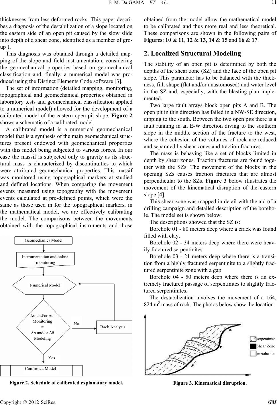
The mass is behaving like a set of blocks limited in
depth by shear zones. Traction fractures are found toge-
ther with the SZs. The movement of the blocks in the
opening SZs causes traction fractures that are almost
perpendicular to the SZs. Figure 3 below illustrates the
movement of the kinematical disruption of the eastern
slope [4].
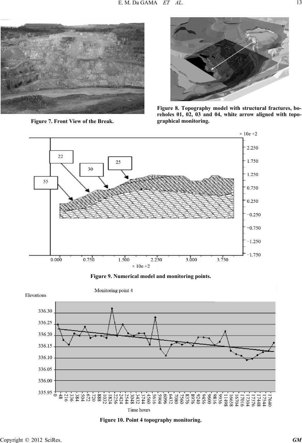
This shear zone was mapped in detail with the aid of a
drilling campaign and detailed description of the boreho-
le. The model set is shown below.
The descriptions showed that the SZ is:
Borehole 01 - 80 meters deep where a crack was found
filled with clay.
Borehole 02 - 34 meters deep where there were heav-
ily fractured serpentinites.
Borehole 03 - 21 meters deep where there is a transi-
tion from a highly fractured serpentinite to a slightly frac-
tured serpentinite zone with a gap.
Borehole 04 - 50 meters deep where there is an ex-
tremely fractured passage of serpentinites to slightly frac-
tured serpentinites.
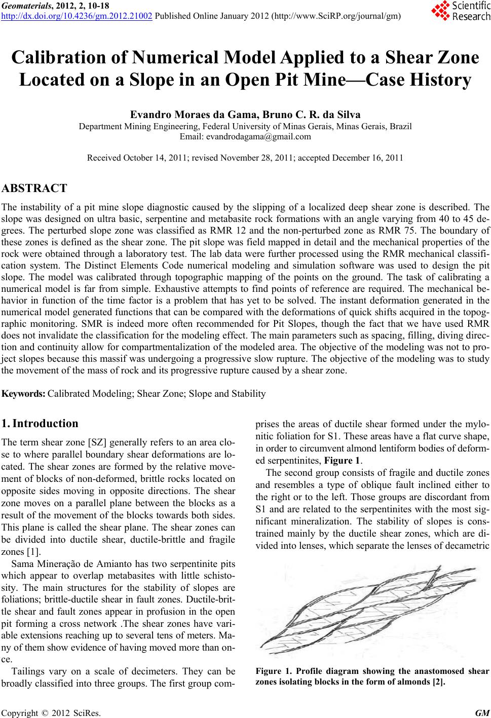
The destabilization involves the movement of a 164,
824 m3 mass of rock. The photos below show the location.
Figure 3. Kinematical disruption.

E. M. Da GAMA ET AL.
12
Figure 4. SZ Shear Zone, boreholes 01, 02, 03, and 04 RMR
= 12 rock mass fractured, RMR = 75 rock mass no fracture.
Figure 5. Slope top disjointed.
Through a detailed description of the fractures with the
aid of detailed topography and measurements taken with
a compass, it was possible for us to build a to-pography
model, adding the mapped fractures.
3. Laboratory Test
There are two geometric areas. The first one is above the
sliding surface (SZ) with spacing between blocks ranging
from 7.0 m to 5.0 m from south to north in an east-west
direction. This is the area which was directly affected by
the landslide. The second one is below the sliding surface
(SZ) with spacing between blocks of about 10.0 m to 7.0
m from south to north in an east-west direction.
Laboratory tests were conducted by IPT Brazil [5], a
benchmark in South America for geomechanical proper-
ties of rocks and Cojean [6] focused on the shear strength,
uniaxial compressive strength using the indirect tensile
strength method. Because the samples did not the have
proper structure to undergo direct tensile strength tests, a
diametral compression or indirect tensile strength, was
applied, as suggested by ISRM—the International Soci-
ety of Rock Mechanics.
The north-south (305/86 SW family—foliation) 66/30
and NW (family of discontinuity) discontinuity rigidity
properties were calculated using the RMR methodology
for the boreholes
The RMR used for the area before the SZ was 12 and,
for the area after the SZ, it was 75. The calculation of the
discontinuity rigidity properties was based on [7].
The UCS of 93.90 MPa refers to the rocky matrix of
the serpentinite with no discontinuities and the cohesion
equal to zero is due to the foliation which is an open dis-
continuity and therefore presents a cohesion of zero with
its resistance attributed to the friction angle of 22.10 de-
grees and Kn stiffness of 249.19 MPa and Kt 95.18 MPa.
The foliation and the 66˚/30 ˚ family NW inside SZ are
within the shear zone and therefore are working with a
cohesion of zero or very near zero. This shows that the
movement is greater through these discontinuities.
4. Calibrated Numerical Model
The numerical model was calibrated using four points
following exhaustive research to identify which points
have displacements similar to the four points which were
topographically monitored. Metal rods introduced into
2-inch holes and equipped with electronic sticks and mo-
nitored with total station. Four topographical points were
monitored for 672 days. The numerical model and mo-
nitored points are shown in Figure 7 below. The topo-
graphic monitoring shown by Figures 6, 8, 10 and 12, is
referenced to topographical coordinates on the y axis and
the x-axis refers to time in hours. The comparisons of dis-
placements commented on below show vertical displace-
ment in metric units. These displacements are variations be-
tween the metric topographic coordinates.
The graphs below, Figures 10 & 11, 12 & 13, 14 & 15
and 16 & 17, show and compare the results gathered at
the monitoring points of topographic displacement and
their respective calibrated modeling points 55, 22, 30 and
25 in Figure 9.
Figure 10 shows the monitoring of topographic point
4 and Figure 11 shows point 30 of the calibrated nume-
rical model. There is a rapid vertical displacement, suggest-
ing the accommodation of the blocks at the most fractured
Figure 6. Ramp access destroyed.

E. M. Da GAMA ET AL.
GM
13
Figure 8. Topography model with structural fractures, bo-
reholes 01, 02, 03 and 04, white arrow aligned with topo-
graphical monitoring.
Figure 7. Front View of the Break.
Figure 9. Numerical model and monitori ng points.
Figure 10. Point 4 topography monitoring.

E. M. Da GAMA ET AL.
14
Figure 11. Point 30 calibrated modeling.
zone of the ramp, which were the largest blocks. The
order of magnitude of the vertical displacements ranged
from 0.13 to 0.32 m.
We observed the same trend in the accommodation
blocks with a vertical variation of between 0.1 and 0.8 m.
The numerical model was not able to show a temporal
variation as the topographic monitoring was. We did no-
tice, however, that the extent to which the 0 to 3 UDEC
cycles are applied determines the vertical displacement
decrease.
Figure 12 shows the monitoring of the topographic
point and Figure 13 shows point 25 of the calibrated nu-
merical model. Section 1, which is monitored via topo-
graphy, shows a maximum displacement of 1.40 m be-
tween 0 and 5616 hours. At two peaks, displacements at
1834 hours and 5616 hours were observed. The dis-
placements and absolute magnitude are located between
0.30 and 0.80 m. These shifts are associated with accom-
modation blocks. After 16,704 hours, shifts are on the
order of 0.25 m with a tendency to remain constant for
some time.
The point 25 of the calibrated model shows two points
of maximum displacement of 0.30 m and 0.15 m. After
being stabilized at 0.25 m, we kept it this way until the
blocks had been stabilized.
Figure 14 shows the topographic monitoring of sec-
tion 2 and Figure 15 shows the corresponding point in
the numerical model.
Between 0 and 1032 hours there is a maximum dis-
placement of 1.1 m. At the 1032nd hour we have a peak
displacement of 1 meter. After this peak, shifts tend to
stay at a constant topographic level (325), and show a
second set of displacements at elevation 324.5. Figure
11 shows point 35 of the calibrated model where we have
the same trend.
There is a rapid increase in deformation to 0.18 m.
Then we have variations of displacement close to 0.18 m.
Finally, the model stabilizes at 0.175 m. This point does
not show an order of magnitude for displacement similar
to the topography and neither do monitoring points 25
and 30. Figure 14 corresponds to the third point of topo-
graphical tracking and Figure 15 shows the correspond-
ing point in the calibrated model.
Figure 16 shows a progressive shift from 1 to 2 meters
over a 426-hour interval, stabilizing at topographic eleva-
tion 332.
From this point we have a gradual stabilization, pos-
sibly temporary, with a maximum displacement of 0.5 m.
Figure 12. Point 1 topography monitoring.

E. M. Da GAMA ET AL. 15
Figure 13. Point 25 calibrated modeling.
Figure 17 corresponds to the numerical model and sho-
ws the same trend. There is a quick shift to 0.09 m after a
gradual stabilization near 0.085 m. But this point does
not show an order of magnitude for displacements simi-
lar to the displacements obtained through the topographic
monitoring.
5. Discussion
The curves for the displacements obtained through the mo-
nitoring show topographic features very similar to the
displacement curves obtained in the numerical model.
Paragraphs 30 and 25 of the numerical model show an
order of magnitude for the displacements that is com-
patible with the numerical model. However, points 55
and 22 do not present an order of magnitude for the dis-
placements that is compatible with the topographic
monitoring.
The topographically monitored points are spaced 100
meters apart. The blocks are disconnected, and their fric-
tion coefficient is the only stabilizing factor. The more
density there is the greater are the friction and the safety.
Thus, the orders of magnitude for the displacements of
points 55 and 22, which were similar to those topogra-
phic monitoring points, should have been on blocks that
were separated or not engaged in the model. But it is not
an easy task to consider all the blocks and choose those
with mechanical behavior compatible with the real mag-
nitudes of the displacements, obtained from topographic
monitoring.
However the interpretation of physical and mechanical
stability is maintained because the curves show displace-
ment functions very similar and comparable to those ob-
tained in the topographic monitoring.
The movements are typical of disconnected blocks
where small deformations accumulate over long periods
and suffer large deformations faster than usual. The fas-
test movements were caused by the dismantling with ex-
plosives of the front slope in the studied area.
It was observed that the size of the displacement of
Figures 6-8 ranges from 0.15 to 0.30 m. Point 4 is in the
highest elevation of the ramp followed by monitoring
points 1, 2 and 3. There is a clear trend towards an incre-
ase in the vertical displacement over time.
Figure 14. Point 2 topography monitoring.

E. M. Da GAMA ET AL.
16
Figure 15. Point 55 calibrated modeling.
The Topography monitoring used did not allow for a
continuous evaluation of the data with shorter time in-
tervals. On the other hand, kn (Normal Joint stiffness)
and kt (Joint shear stiffness) applied to the model, can
impose minor displacements between the blocks. All
these factors make the numerical calibration of the model
more difficult [4].
The numerical modeling was performed using the
UDEC: Universal Distinct Element Code software, ver-
sion 3.0 Itasca Consulting [8].
5.1. Input Data and Assumptions in the Model
The model was based on the size of the blocks in Figure
4. The results of the field mapping were used for the
biggest blocks which have dimensions (in meters) of 6.20
× 4.50 × 5.20 × 2.30 and 4.60 × 2.80. The input parame-
ters for a numeric geomechanical model are the me-
chanical properties shown in Table 1 and the discon-
tinueties mapped in the field. As a synthesis of a struc-
tural model, the model presented may appear simple.
However, the complexity of this model lies in the fact
that there is a numerical convergence of the results.
5.2. Results
In Figure 18 the dark lines show the model simulation of
the slip surfaces of slope, which are within the friction
limits, or that is those that are collapsing. They indicate
that the SZ, represented by the thick, dark line is found in
the process of collapsing. The same occurs at several
points of the 66/30 NW foliation family, which are also
in process of free shear.
Figure 19 shows that, through the simulation model,
maximum displacements of 4.41 × 10−2 m were found,
which are represented by the regions highlighted by the
thick, dark lines. At such discontinuity points, the dis-
placement opens and continues moving.
Figure 16. Point 3 topography monitoring.

E. M. Da GAMA ET AL. 17
Table 1. Results of mechanical laboratory tests.
Lythotypes C
Mpa
Φ
grade
σc
Mpa
σt
Mpa
γ
t/m3
G
Mpa
K
Mpa
Kn
Mpa
Kt
Mpa
Serpentinite Matrix 1.10 44.90 93.90 11.07 2.63 17521.00 37963.00
Foliation inside SZ 0.00 22.10 249.18 95.81
66˚/30˚ Family NW inside SZ 0.09 29.60 249.18 95.81
Foliation after SZ 0.26 26.90 4047.82 1553.60
66˚/30˚ Family NW after SZ 0.97 58.50 4047.82 1553.60
C: cohesion, θ: friction angle, σc: Uniaxial Compression , σt: Indirect Tension, γ: density, G: Shear modulus, kn: Normal Joint stiffness, kt: Joint shear
stiffness.
Figure 17. Point 22 calibrated modeling.
Figure 18. Joint now at shear limit shown in darker lines.
6. Conclusions
The destabilization of a shear zone, shown in this paper,
is a slow and continuous process.
Topographic monitoring, especially from point 04
when compared to the 30th point shows a weak relation-
ship with the displacement of the surface of the tracked
slope and a small similarity to the numerical model de-
veloped.
Factors contributing to this destabilization are closely
linked to the angles of the slope used in the plowing op-
erations and placement of embankments with a geometric
relationship to the fault and SZ located near the face of
the dismantled slope.
This analysis shows the need for a detailed map of the
structural stability of the open pit in operation.
The task of calibrating a numerical model is far from
simple. Exhaustive attempts to find points of reference
are required. The time factor is a problem that has yet to
be solved, but, for now, the deformation generated in the
Figure 19. Shear displacement show n in dar ker lines.

E. M. Da GAMA ET AL.
18
numerical model generated functions that can be com-
pared with the deformations with quick shifts acquired
through topographic monitoring.
The topography does not allow for the tracking of a
continuous data record. With a continuous record of, for
example, one measurement per minute, perhaps we’d
have a better calibration of the model [9].
REFERENCES
[1] J. G. Ramsay, “Shear Zone Geometry a Review,” Journal
of Structural Geology, Vol. 2, No. 1-2, 1980, pp. 83-89.
doi:10.1016/0191-8141(80)90038-3
[2] Y. Hasuo, F. S. Magalhaes and A. F. Mangolin, “Applied
Structural Geology,” 1992, pp. 363-382.
[3] P. A. Cundall, “Numerical Modeling of Jointed and
Faulted Rock in Mechanics of Jointed and Faulted Rock,”
A. A. Balkema, Rotterdam, 1990, pp 11-18.
[4] E. Gama and L. Borrher, “Efeito de uma zona de
cisalhamento na estabilidade de um talude de mineração”.
In: IV Congresso Brasileiro de mina á ceu aberto e mina
subterranea, Belo Horizonte. MG Brasil, 2006.
[5] IPT, “Relatório de Ensaios,” Instituto de Pesquisas
Tecnologicas, Sama Mineração, 1996.
[6] R. Cojean and S. Curtil, “Rapport d’Avancement des
travaux de Thése,” ARMINES Centre de Geologie de
L’Ingenieur, Paris, 1995.
[7] P. A. Cundall and R. D. Hart. “Development of General-
ized 2-D and 3-D Distinct Element Modeling Programs
for Jointed Rock,” Itasca Consulting Group, US Army
Corps of Engineers, Itasca Consulting Group, 1985.
[8] D. Billaux, F. Dedecker and P. Cundall, “A Novel Ap-
proach to Studying Rock Damage: The Three Dimen-
sional Adaptive Continuum/Discontinuum Code,” Pro-
ceedings of EUROCK 2004 & 53rd Geomechanics Col-
loquium, Ed. Schubert, 2004, pp. 723-728.
[9] E. M. Gama. “Rock Mechanics Applied to Mining,”.
EEUFMG, Vol. 1, 2005.