Received 8 October 2015; accepted 28 December 2015; published 31 December 2015

ABSTRACT

The consequence of the 5D projection theory [1] is extended beyond the Gell-Mann Standard Model for hadrons to cover astronomical objects and galaxies. The proof of Poincare conjecture by Perelman’s differential geometrical techniques led us to the consequence that charged massless spinors reside in a 5D void of a galactic core, represented by either an open 5D core or a closed, time frozen, 3D × 1D space structure, embedded in massive structural stellar objects such as stars and planets. The open galactic core is obtained from Ricci Flow mapping. There exist in phase, in plane rotating massless spinors within these void cores, and are responsible for 1) the outward spiral motion of stars in the galaxy in the open core, and 2) self rotations of the massive stellar objects. It is noted that another set of eigen states pertaining to the massless charged spinor pairs rotating out of phase in 1D (out of the 5D manifold) also exist and will generate a relatively weak magnetic field out of the void core. For stars and planets, it forms the intrinsic dipole field. Due to the existence of a homogeneous 5D manifold from which we believe the universe evolves, the angular momentum arising from the rotation of the in-phase spinor pairs is proposed to be counter-balanced by the rotation of the matter in the surrounding Lorentz domain, so as to conserve net zero angular momentum. Explicit expression for this total angular momentum in terms of a number of convergent series is derived for the totally enclosed void case/core, forming in general the structure of a star or a planet. It is shown that the variables/parameters in the Lorentz space- time domain for these stellar objects involve the object’s mass M, the object’s Radius R, period of rotation P, and the 5D void radius R_o, together with the Fermi energy E_f and temperature T of the massless charged spinors residing in the void. We discovered three laws governing the relationships between R_o/R, T, E_f and the angular momentum Iω of such astronomical object of interest, from which we established two distinct regions, which we define as the First and Second Laws for the evolution of the stellar object. The Fermi energy E_f was found to be that of the electron mass, as it is the lightest massive elementary particle that could be created from pure energy in the core. In fact the mid-temperature of the transition region between the First and Second Law regions for this E_f value is 5.3 × 10⁹ K, just about that of the Bethe fusion temperature. We then apply our theory to analyse observed data of magnetars, pulsars, pre-main-sequence stars, the NGC 6819 group, a number of low-to-mid mass main sequence stars, the M35 members, the NGC 2516 group, brown dwarfs, white dwarfs, magnetic white dwarfs, and members of the solar system. The ρ = (R_o/R) versus T, and ρ versus P relations for each representative object are analysed, with reference to the general process of stellar evolution. Our analysis leads us to the following age sequence of stellar evolution: pulsars, pre-main-sequence stars, matured stars, brown dwarfs, white dwarfs/magnetic white dwarfs, and finally neutron stars. For every group, we found that there is an increasing average mass density during their evolution.

Keywords:

Origin of Mass and Self Rotation of Stellar Objects, Angular Momentum, Fermi-Dirac Distribution

1. Introduction

Two years ago, a 125 GeV p-p resonance was forwarded as the probable proof of the existence of the Higgs boson condensed vacuum [2] . About that same time, in view of the proven Poincare Conjecture [3] [4] using differential geometrical techniques (particularly the Ricci flow theorem) developed over the past decade [5] -[8] , we proposed a grand unified field theory. From such research, it was found that the p-p 125 GeV state is directly deducible from that theory without requiring the existence of a condensed Higgs Boson vacuum. This grand unified theory is based on the dimensional projection actions of the 5D homogeneous space-time onto the 4D Lorentz space-time [1] [9] . Before we apply the 5D projection theory, we first briefly review the essence of the theory below. The Poincare conjecture states that all 3D manifolds can be projected into a sphere. Starting from a 5D homogeneous space-time, Perelman showed that through Ricci Flow mapping (in differential geometry), one obtains a 4D Lorentz manifold. This Lorentz 4D covariant space-time is not 3D coordinate homogeneous―rather it has the geometric shape of a doughnut. It is noted that the center of the doughnut shaped Lorentz manifold is in 5D, and the top and bottom of this doughnut center can be closed into a line passing through the Lorentz domain. The projection process is then followed by a translation displacement of the lines to the inner surface of the 5D core domain, making it into a closed loop, and thus fixing the time to a fixed value, giving the core as a 3D × 1D time fixed manifold. The 3 coordinates in Lorentz space become homogeneous. Thus any matter within this representation is spherical in shape, satisfying the Poincare Conjecture. In the quantum projection theory [1] the Lorentz manifold can be obtained from two orthogonal projections. One is a space to time projection Po, which gives rise to the result of SU(2) × L manifold, and the other is a space to space conformal projection P1, which gives rise to the result of SU(3) × L manifold, via 5D to 4D mapping; L is the Lorentz space-time. Here × represents a direct product of the two groups. It is these 2 orthogonal manifolds that allow for the realization of massive leptons, and quarks. However, the formation of hadrons from gauge confinement of quarks requires the Gell-Mann quark standard model [10] , which consists of 3 pairs of (−1/3)e, (2/3)e quarks, not just the SU(3) generators (i.e. (2/3)e, (2/3)e and (−1/3)e). The two (2/3)e charges belong to two different quarks that form part of the SU(3) generators. Such a difference implies that the symmetry of SU(3) is broken, hence allowing for the superposition of Po and P1. It is this realization that allows for the quantization representation of the Perelman-Poincare projection, which is employed in our stellar rotation model in this paper.

Through several follow-up articles [11] -[13] it was further shown that hadron masses can be calculated accurately based on the requirement of gauge invariance, of which the 125 GeV p-p state is realized. Analyzing the possible type of field solutions to the quantized homogeneous 5D metric equation that must exist in the homogeneous 5D domain, we found solutions representing (a) massless spinors with opposite charges, and (b) electromagnetic fields represented by Maxwell vector potentials. Since the product of (a) and (b) is also a (field) solution of the metric operator, and following gauge transformation, the coupling constant is then designated as the electronic charge e which can take on positive and negative sign; such a coupling constant is then considered to be the origin of the unit charge e in the universe (see Chapter 4, and Chapter 7 of [1] ). Furthermore, this coupling between the two field solutions is decoupled by a gauge transformation, through the establishment of the unit flux quantum (h/e). It was then shown mathematically that through dimensional projection, massive fields will be created into the Lorentz manifold, leading to the emergence of the Lorentz Riemannian geometry. Therefore, the superposition of Po and P1, is required also for establishing the Riemannian 4D space-time needed for Einstein’s gravity equation. Through the derivation of the resultant SU(3) × L, the Gell-Mann standard model [10] of quarks was retrieved, leading also for the first time, to our ability to formulate the gluon potentials generated by quark currents in the structures for mesons and for baryons [11] [12] . The success of the above for understanding the Standard Model, provides us some concrete support to the projection theory of 5D space-time. With the above brief background, the following statement can be considered as the basis of our model for analyzing the origin of mass and angular momentum of stellar objects in this paper. Taking P as the equivalence to Perelman’s mapping, it was then found that the Poincare conjecture of mapping the 4D Lorentz space-time can be transformed into a spherical 3D structure, except that there will exist a fully enclosed time frozen, 4D space void, represented by 3D × 1D, where the 3D is a spherical volume, with radius R_o. Hence we shall refer R_o as the radius of the 4D space void, with time fixed, such that massless spinor states are perpetual, unless thermal energy exchanges between the Lorentz boundary and the void core, inside the Lorentz space-time shell, is implemented.

As we have a spherically shaped mass stellar object model enclosing a 3D × 1D void filled with charged massless spinors satisfying the Fermi distribution, we can connect the physical quantities of the thermal bath of the Fermions in the void and the physical quantities of the matter shell, leading to the discovery of the 1st and 2nd Laws regions for these spinors states. This 4D Riemannian space-time obtained from the superposition of both SU(2) and SU(3), is hence given by [SU(2) + SU(3)] × L, as shown in [1] .

Note that the projection from the 5D space-time onto a 4D Lorentz space-time using the Ricci Flow Theorem, produces a Lorentz 4D, without further mapping the 3D space volume in a doughnut shape, while the doughnut center void remains in the 5D manifold. However when the doughnut 3D volume is transformed by further mapping into a spherical shape, the original 5D void at the center is enclosed into a 4D space void, with time frozen, such that any massless charged spinor states within it must be perpetual. However the Maxwell vector potentials can exist in both 5 and 4 dimensions [1] . Thus there exists a mechanism through the diffusion of photons that the massless charged spinors within the 3D × 1D void can in fact exchange energy with its enclosing Lorentz space-time domain. Due to the homogeneity of the 5D space-time, each of the net charge and angular momentum must always be zero. Hence, within the 3D × 1D void, equal amount of + and –e massless spinors must exist. Therefore if through Po projection, some –e massive charges are created in L, then a net equal amount of + e charges must be also created simultaneously by P1. If the combined projection P gives rise to a spherical space volume shell (in Lorentz manifold), then it must contain mass. Since a time independent 4D center void (in 5D manifold) exists, the emergence of any angular momentum L_z in the void by in phase circulation of the oppositely charged massless spinors, an opposite angular momentum―L_z must be generated in the Lorentz spherical mass shell, in order to preserve total zero angular momentum value. In the astronomical scale for stars, this L_z leads to a repulsive potential within such a void, leading to the elimination of the gravitational singularity, similar to the action of the gluon repulsive potential within hadrons [1] . Solutions to a differential equation are defined by the boundary conditions imposed on them. Thus the massless spinors and vector solutions within the void are completely determined by the Lorentz boundary that encloses them. Therefore from the void spherical geometry, the massless charged spinors eigen states, the e-trino and anti-e-trino pairs are rotating along the latitudes and longitudes of the void, occupying a 4D dimension space (out of the 5D manifold, with time frozen) represented by 3D × 1D manifold. This structure gives us a model of the origin of angular momentum, dipolar magnetic field and masses of the stellar objects observed in the Lorentz manifold. In this paper, we aim at obtaining information about the temperature and angular momentum of such spinor pairs by analyzing the observed /deduced angular momentum and other physical parameters of the massive shells of stellar objects, including different types of stars and planets.

After an introduction of the basic concept 5D to 4D projection above, we follow in Section 2 to present a description of the boundary condition at the 5D - 4D “inter-phase”, leading to a brief sketch of the creation of the universe in view of SU(2), SU(3), and 4D Lorentz group representation. Section 3 is devoted to the derivation of explicit formula (expressed as a number of convergent series of E_f/kT) for the angular momentum generated by the spinor pairs rotating in phase. As each type of the spinors is a Fermion system, and the lightest lepton mass energy created by the Po projection is electron, we take the Fermi energy of the spinor to be E_f = 0.5 MeV. The radius of the void R_o is expressed as an explicit function of the shell mass M, with period of rotation P, and observed radius R together with the Fermi energy E_f and temperature T of the massless spinors inside the void core. From this mathematical result, we discovered three laws consequential to the projection theory: 1) At very high temperature such that the angular momentum Lz of the object is mainly contributed by the massless spinors with energies much greater than E_f, the normalized void radius R_o/R is a linear function of 1/T, with a negative slope, which must represent the early stage of the stellar objects. We call this region the First Law region of angular momentum. 2) At relative low temperature kT = E_f, the ratio ρ = (R_o/R) of the object is a linear function of 1/E_f, and not a function T; thus the ρ versus T relation is a horizontal line. We refer this region as that of the Second Law. Hence, this region must describe the last stages of the stellar object. 3) The “mid-temperature” T_c in the transition region between the two laws is a universal constant, dependent only on E_f = 0.5 MeV (which is a universal constant in our theory). We name this as the Third Law. These three stages represented by the three Laws are actually shown in this paper to be satisfied by many known stars classifications. Following, in Section 4, we explain why magnetars/pulsars are new-born stars with detailed numerical illustration of some pulsars examples. Combining with the stellar object’s mass density, we open up an analysis of the angular momentum of star groups according to different ranges of mass density of these stellar objects in Sections 5 and 6, and compare the calculated results with many numerical data examples to support the theory. In particular, we analyze numerically the R_o-T, and R_o-P relations with reference to the general different stages of evolution of these objects. Neutron stars are proposed to be the very oldest stars in Section 7, accompanied with detailed model numerical examples. From purely the view point of angular momentum, planets are similar to stars (see Section 8), but only with smaller values of ρ = R_o/R. A general discussion is presented in Section 9, including a summary of the theory presented focusing on some relevant physics concepts involved, giving a sketch of stellar evolution―from pulsars to neutron stars, and providing simple discussions on the Fermi energy, heat bath, degeneracy of an electron gas, as well as possible Bose-Einstein condensation involved in the final stage of stellar objects. The origin of the stellar magnetic field is only very briefly introduced, as we left that discussion to another paper.

2. A Brief Sketch of Creation of the Galaxies According to the 5D Model―With Photons as the Medium of Energy Transport

Based on the 5D projection theory and Gell-Mann standard model, we put forth the notion that the final major amount of hadron mass comes from Gluon, not from the quark bare masses. The hadrons can only form after grouping through quantum gauge confinement, which must happen sequentially after the existence of quarks on the boundary of the 5D manifold [14] . While hadrons form on the Lorentz 4D boundary, the energy within the 5D domain is carried by the charged massless spinors (fermions) and the vector potentials, which are represented by the photons (bosons). The relation between this energy and temperature, according to quantum statistics, is described individually by the Fermi-Dirac (for the spinors) and Bose (for the photons) distributions respectively. Since the temperature in the void is normally much higher than that of 5D-4D boundary, thermal cooling inevitably takes place via heat diffusion; this rate of cooling progress follows the Navier-Stokes diffusion equation as well as known nuclear, atomic and chemical reactions in sequence: First by Bethe fusion―heavier and heavier nucleons are formed, starting with protons and neutrons, then followed by alpha particles, etc. Second, further energy cooling occurs when the nuclei combine with leptons, mainly electrons, to form atoms. Lastly, as these new and heavier atoms on the boundary within the expanding Lorentz space-time boundary layer forms molecules and then crystal compounds through chemical binding, the boundary surface builds up mass, while thickening.

From the view point of group symmetry, we would like to point out that the boundary of the finite 5D homogeneous manifold must be obtained from a dimension projection, just like the boundary of a 3D space volume is obtained from a 2D projected surface. Hence this 5D boundary is represented by [SU(3) + SU(2)] × L; here L is the 4D Lorentz space-time. It is this topological realization that dictates the special property that the boundary is being composed of net charge neutral masses, starting with quarks and leptons right at time 0, way before formation of hadrons, etc. Such a property must be maintained as the Lorentz 4D domain and 5D both expand through the continuous rebalancing of energy between them.

In field theory, energy can only be carried by quantum fields irrespective of the domains they belong. However, only photons, meaning vector potential fields can exist in both 5D and 4D manifolds. Thus it must be the photons that act as the medium of energy transport between matter fields in L, and charged massless spinors in 5D. Such a diffusion process between energy exchange of 5D to L and vice-versa obeys entropy theorem and violates time reversal symmetry. However, as the unidirectional time and space expansion is built-in from the homogeneous 5D metric, entropy would naturally be obeyed, leading therefore to the statistical thermodynamic theory of nature. In fact it is the application of this entropy law that provides ground of validity for the second step of the Perelman mapping in his proof of the Poincare Conjecture.

For a stellar mass object, the 5D domain within the Perelman-Poincare void core is frozen in time at t = τ₀, thus with or without energy transfer, the expansion in space-time domain occurs only in the L domain surrounding the void core. The opening of the L domain provides a model for the formation of a galaxy, that contains many masses (which we call stars and planets), created by the Ricci Flow of Perelman’s mapping. The galaxy expands in the form of a doughnut 3D space manifold. As the galactic center is in 5D, the galaxy is imbedded in the homogeneous 5D universe. Many galaxies can be created at the same time, on the finite surface area of the so called Creation instant of the 5D manifold. For an averaged galactic core dimension of 100 light years across, it is easy to estimate, based on the domain represented by the Lorentz 4D boundary to the 5D finite domain, that a million galaxies can be simultaneously created by packing the 5D galactic cores together as the entire 5D universe expanded according to the 5D metric from 0 to 1000 light years. Since the centers of the galaxies are connected in the 5D enclosing domain, light can be transmitted between these doughnut galaxies; hence an event at any one point in one Galaxy can be observed by observers in its own, as well as those in other galaxies. A 1000 years is very short as compared to the estimated age of the Milky Way galaxy. Thus if all galaxies were created simultaneously by the Big Bang, then the universe’s age is close to the galaxies age as conjectured by some scientists.

Note that the boundary of the entire 5D universe is represented in terms of the product of three groups: SU(2), SU(3), L, and thus must contain quarks and leptons, plus the 5D voids. Hence, as the universe expands, the density of these massive charges on the boundary of the universe must continue to reduce as the 5D expands, leading to a condition that allows us to treat the entire 5D universe encompassing interior fields of both massive objects and massless vector and spinors to be solutions of the 5D and Lorentz’s metrics operators with open boundary condition. As the 5D space and time dimensions increases, due to the uncertainty principle, with the key parameter specified by the Planck’s constant h, the 5D domain becomes very large, and the fields in the 5D domain will become classical with continuous eigen spectrum energies. Hence astronomical objects obey classical laws, except for neutrinos. The observation of neutrino oscillations and its theoretical explanation is a clear illustration of this boundary effect [9] [15] .

Because of the increase in mass distribution throughout the Lorentz space-time of all created matters, the Riemannian curvature also continuously changes, leading to the increase in the gravitational contracting force acting on the massive shells of stars. Whereas stars with masses smaller than the Chandrasekhar limit will shrink to dwarfs of various colors, those with mass > 1.4M_Θ undergoes gravitational collapse eventually to form neutron stars; more details will be followed up in later sections. The initial formation of a matter shell occurs at extremely high temperatures (see Section 4), and the heat loss to the L thermal bath from the spinor void via diffusion takes a long time. At the very initial formation of 5D space-time, the amount of starting energy is almost infinite, while all the cooling processes take a very long time as the domain expands indefinitely according to the homogeneous 5D metric. In fact, it is this ever expansion of the universe according to the metric, that induces the establishment of statistically generated ensemble theory from which thermal dynamics is realized, with the 5D-4D boundary acting like the wall of a heat bath container.

We may also look at the creation process in terms of the space-time and parity nature of the 5D metric, as if each star starts from a completely new 5D. Such a picture is possible, as 5D is finite with no absolute center point, and can be created from absolute NOTHING. Hence multiple 5D can be created at the Big Bang instant, but these domains must be merged into one eventually. The interesting aspect lies in their boundaries that distinguish them! Each boundary is in a 4D Lorentz domain, characterized by their different quarks and leptons mass values! Hence from Perelman’s mapping, these different Lorentz 4D domains (or one unconnected form of 4D Lorentz boundary) are represented by the different galaxies, within each, via Perelman’s mapping, is further separated into stars and planets, having individual 5D void cores. Depending on the core sizes, and in view of the uncertainty principle, different amounts of energy are created within individual 5D cores. Such amounts of energy are represented in terms of the energies of the massless fields, namely the vector potentials and e-trino, anti-e-trino spinors. Through these massless fields, the L_z of the quarks is generated in the Lorentz 4D domain(s). In this sense, we may view the above process as the Big Bang creation of the Universe. However, the mass thus generated was not the final amount of mass in the universe. The total mass is actually changing, as the Gauge Constraint converts multiple quarks into hadrons, then into nuclei via Bethe fusion, and to atoms via Coulomb potential, (including 2D Chern-Simons hydrogens), then via Van der Waal potential to molecules, to gases, and crystals. The above-mentioned series of process of formation is a continuous thermodynamic process, via the continuous application of the Law of Entropy, which is built in by the “non-time reversal” nature form of the 5D metric itself. In another word, the act of projection was automatic due to the very nature of the finiteness of the 5D metric, requiring no further action from the creation process. All the amazing complexities of the Universe hence evolve by itself from the beginning based on the homogeneity of the 5D manifold. Each state―change obeys causality, giving raise to even complex life forms, that would also self evolve―with determination to its own future. In another word, the continuous thermal evolution, when applied to life forms, i.e. Darwin evolution, can be viewed also as part of the evolution of creation of matter in the Lorentz space-time.

We will proceed to derive explicit representations of the angular momentum of the 5D structure inside the void over a wide temperature range, and apply the consequence to analyze different types of stellar objects in later sections.

3. The Three Laws of Angular Momentum Generated by in Phase Massless Charged Spinor Pairs Rotating along the Latitudes of the 5D Void of the Galactic Core, and 4D Space Void in Stellar Objects

Consider a system of particles in thermal equilibrium in the void. The density of quantum states within elementary momentum dp and elementary real space dr in the 3D spherical void is gs∙g(p)dr∙dp, where gs measures the spin degeneracy and g(p) is the number of states per unit momentum range. As the quantum unit in phase space

(r, p) is h³, the total number of quantum states within the volume of interest is.

Since the void is a sphere with radius R_o,.

(3.1)

As the 5D metric (represented by (ct)² = x², where x is a four-vector) is homogeneous, when the projection action is taken at t = τ₀, the 4D space volume (out of the 5D manifold) as represented by x² is fixed, though the shape may take any “close” form. As the 4D space void is enclosed by the Lorentz space-time, which has only 3 space coordinates, the 4D space void must be expressible as 3D × 1D, and all components of x are equal, with the void radius R_o being fixed. Note that a similar statement cannot be applied to the energy-momentum metric E² = (cp)², because action of projection is not taken at fixed E value. We would also remark again that when mass is created due to projection action, a Lorentz boundary is formed, enclosing the 3D × 1D void. Due to 3D spherical symmetry, all eigenstates of spinors within the void must be represented by spherical symmetric functions, namely L' (quantum states pertaining to spinors rotating along the longitudes, not relevant to nonzero angular momentum generation here), and L_z (angular momentum due to spinors rotating along the latitudes). It is the net L_z that will lead to the mass shell rotation, such that the total angular momentum in the whole universe (including 4D and 5D) remains zero at all time, as explained in the Section 1. The spinors are Fermions, but of opposite charge, and are strictly speaking, of different kinds of Fermions, which follow the relevant statistical distribution(s). The Fermi-Dirac L distribution, which is expressed generally as

(3.2a)

where s is the normalization factor, and L_f is the “Fermi angular momentum”, satisfying the property that the probability is unity for angular momentum smaller than L_f, but is zero for L > L_f at temperature T = 0 K. Since L = (2hν/c)R_o = 2Eτ₀ at time τ₀ (here ν is the frequency), we define the Fermi angular momentum to be L_f = 2E_fτ₀. The normalized factor s is simply kτ₀ so that Equation (3.2a) becomes

(3.2b)

where k is the Boltzmann constant.

The Fermi distribution in (3.2b) now describes a pair of spinors. For pairs of such spinors in the void rotating in-phase so that each pair has zero charge, the angular momentum generated along the spin axis z by spinor pairs rotating along the latitudes of the void, weighted over the Fermi distribution (pair), is

(3.3a)

where r' = r∙sinθ, and θ is the polar angle and ψ is the azimuthal angle so that all spinor pairs generating L_z within the void are counted. θ is integrated from 0 to π, and ψ is integrated from 0 to 2π (to avoid over-counting because there are orbits along the longitudes). After integrating over r, θ and ψ,

(3.3b)

where z is the unit orientation vector for L_z. Noting that p stands for the momentum of a pair, giving, , and we arrive at

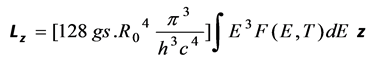(3.3c)

It is shown in Appendix A that the above integral can be expressed as a sum of a number of series, so that we have simply

(3.4)

where = E_f/kT

(3.5)

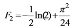
For very small = 1, it is shown in Appendix B that

, (3.6a)

where, with gs = 4, and L_z is independent of. On the other hand, for large » 1, we simply have (Appendix B),

, and hence L_z is independent of T (3.7a)

For intermediate values of, we need to calculate

(3.8)

We name Equation (3.6a) as the First Law, Equation (3.7a) as the Second Law of Angular Momentum, resulting from the 5D projection theory quantum statistics. L_z is to be equated to the mass shell angular momentum Iω of the matter object, where I is the shell’s moment of inertia, and ω is its rate of rotation about the unit vector z, as measured or deduced from astronomical studies. Thus the First Law can be expressed as,

(3.6b)

where A = D^−0.25{7π⁴/1920}^−0.25 = 4.52 × 10⁻¹⁸ S.I. units. While according to the 5D projection mapping, the void is fixed at t = τ₀, thus the void has a radius R_o = cτ₀. Hence, the Second Law can be expressed as

(3.7b)

Dividing Equation (3.6b) by Equation (3.7b), we arrive at

(3.9)

For fixed E_f, the “mid/critical temperature” T_c of the “transition region” (that between the First and Second Laws) can be found using (3.9). For example, if we take E_f = 0.5 Mev, T_c = 5.3 × 10⁹ K. We may consider (3.9) as the Third Law, which is universal according to the 5D model. As the First and Second Laws have simple linear relationships, is just the intersection of two straight lines. In other words, this particular point shows the location where the two linear lines would have met if each law has its ultimate linear form. However, ρ is dependent on E_f in the Second Law region and gives us information (with reference to E_f, T) about the temperature of the transition region for each E_f value.

Hence we must determine the E_f value for application. From the 5D E, p metric, with the projection into SU(2) × SU(3) × L, the lowest mass value is that of the electron’s rest mass m_e. Thus we have the condition E² >. In view of this minimum energy principle, the value of E_f is chosen as 0.5 Mev, indicating that the lightest lepton is generated (see Sections 1 and 4 for more details).

4. Formation of New Born Stars―Pulsars According to the Projection Theory

The mapping of the 5D space-time into a 4D Lorentz space-time (represented by general projection P) using the Ricci Flow Theorem, produces a 3D space of a doughnut structure containing matter, but enclosing a void core (in 5D space-time). It has been noted that P can be represented by a combination of the space to time projection operator Po (or time shift operator) and the space to space conformal projection operator P1. From these projections we obtain the “key stable elementary particles” which build up matter in the 4D Lorentz space-time. These particles are electrons, protons, and neutrons. Keeping in mind that the protons and neutrons are built by quarks, which are fractionally charged. Using a 2D circular coordinate transformation as a simplified example, it has been explained in [12] that Po would lead to creation of leptons which satisfy the SU(2) symmetry and P1 would give rise to the existence of the quarks that satisfy the SU(3) symmetry. It has been inferred that Perelmann’s projection theory based on Ricci flow concept in differential geometry would lead to the same conclusion [1] . Since the Lorentz boundary domain must be charge neutral if the 5D is homogeneous, thus the void, open or enclosed must be charge neutral, and if charged massless spinors exist in 5D, due to charge conservation, equal number of massless spinors with opposite charges would exist in the 5D manifold [chapter 6 of 1]. When mass is created, a boundary exists between the void and mass structure outside. As explained in Section 1, the in phase circulating pair states of spinors will produce a net angular momentum L_z, with the spinning axis z perpendicular to the doughnut/sphere plane (of the galaxy). Hence to conserve angular momentum, the matter in the sphere must move in such a way as to generate the same amount of total angular momentum, but rotating in the opposite sense (i.e. –L_z).

In view of SU(2) symmetry and energy consideration, for every lepton creation with a net charge e, a massless and charge-neutral neutrino must also be created to conserve zero spin. It was argued in [1] that as an anti-neutrino is chargeless, it cannot be coupled to the vector potential anywhere. A hypothetical anti-neutrino must obey the exact same boundary condition as the neutrino if a solution exists; however, such a solution is not different to that represented by the neutrino. Hence there is an asymmetry between neutrino and anti-neutrino in the SU(2) representation. The above statement essentially means that the SU(2) representation resulting from Po projection breaks time reversal symmetry. Therefore there are only leptons with negative e charge with its neutrinos in the 4D space time, and thus the universe does not contain anti-matter symmetry. Incidentally the charged leptons are: the electron (e) and the highly unstable, but heavier versions of electron-muon (μ), the tauon (τ). While the neutral leptons are the (electron, muon, tau) neutrinos. Among those charged leptons, electron has the lightest rest mass of 0.5 MeV. Within the time frozen, 4D space void, the massless charged spinors appear in pairs, and the minimum “energy expenditure” of these spinor pairs in the Po projection to create matter with mass is therefore at least of 1 MeV; we can consider such a property as also due to gauge symmetry. Thus Po projection leads to the creation of 2 electrons running in opposite directions (plus neutrinos) as the most stable leptons in the star. Through Po projection, though other members of the leptons were also created, yet these are very unstable, and will not remain in the massive Lorentz boundary. Note that the metric of the totally enclosed void, within a stellar object, is represented by a 3D × 1D space, with time frozen when the enclosing Lorentz boundary is static (Poincare-Perelman projection/mapping). However, the general entropy theorem requires that this boundary will exchange energy with the void core, hence changing the void representation to 3D × 1D × time, which in turn induces the grow of the Lorentz boundary shell (Einstein-Stokes relation, see [16] ). At the same time charge neutrality must be maintained. Via Po, only negative charges are created, and an equal amount of positive hadrons must be created (via P1) within the Lorentz boundary domain. As quarks are generated via conformal projection P1 from 5D to the 4D space-time, and due to the gauge invariance property, positive hadrons can be formed. Thus the charge neutrality requirement can be considered as the reason why Po and P1 must be enacted simultaneously. Members of the quarks have either positive or negative fractional electric charges. When they obtained their masses by quantum confinement, positively charged protons will appear in the Lorentz space-time with number equal to that of the electrons, conserving overall charge parity in the 4D universe. The interaction of the gluon potentials (in Lorentz space) and the vector potential (in the 5D void) has been explained in Section 1. Hadrons can be separated into two sub-families: baryons (the most stable ones are protons and neutrons) which are built of three quarks. On the other hand, each of the mesons (such as pions) belonging to the second sub-family is built of one quark and one anti-quark. Therefore the combination projection P0 and P1 leads to the creation of all the elementary particles detected/perceived in the 4D manifold in which stars are observed to exist. These particles form a shell enclosing the void. As projection/creation goes on, the shell increases its mass and thickness. Since the temperature at this stage of a star is extremely high, at the beginning, the individual quarks might exist, together with the gluon potential fields. It takes a long time before the right combination of the quark members to become confined by gauge and to form hadrons, at the same time emitting large amount of energy in a wide range of the electromagnetic spectrum; such radiations are observed from pulsars (see e.g. [17] ). Note also that due to Chern-Simons gauge property [12] [18] -[20] , the quark-current will rotate in a 2D manner on top of this early stage thin mass shell, generating huge magnetic field (with axis not necessarily along the L_z direction) of a new born star. Such huge electromagnetic fields are observed in pulsars and magnetars. Other models have also proposed the idea that enormous amount of electromagnetic energy is radiated from the outer-shell from a typical pulsar (see e.g. [21] [22] ). In fact, models suggesting strong gamma radiation near the centre of the galactic core have been proposed, as emitted by pulsars [23] . We propose that magnetars (stars with surface magnetic field ~10¹⁰ - 10¹¹ Tesla; (see e.g. [24] ) are the youngest new born stars, and pulsars are the “elder ones” of these young baby stars according to the model resulting from the 5D to 4D projection. The readers are referred to [25] for useful data of pulsars. Other theories have argued that the temperature of pulsars is greater than 10⁹ K, happens to be consistent with our Third Law [26] [27] . In this paper, we do not analyze the magnetohydrodynamics of the pulsar atmosphere as in [28] since the process is very involved, and model-dependent. We would only study the plausible consequence of the projection theory based on fundamental physics laws. In passing, we point out that there is observation of large mass structure ~10⁴ solar mass near the centre of a galaxy, and there are numerous young stars near the galactic centre also [29] . Generally, it has been believed that the strong magnetic field of pulsars/neutron stars originated from the collapse of the core of a supernova with the conservation of magnetic flux (see e.g. [30] ). Here we have provided another possible explanation of the origin of the huge magnetic field based on the existence of surface quark currents of these stars. We would draw attention to the recent finding that even though pulsars have different magnetic field intensity and a wide range of rotation rates, the γ-ray spectra of young pulsars are similar, fitting a hard power-law with a modified exponential cutoff [31] .

We would like to remark also that at the birth of a star, there is relatively small amount of (massive) matter, and the electrons and quarks must spin very fast in order to counter-balance the angular momentum of the spinor pairs within the 4D space void of the young star. To form a baryon, the right quark members must be combined in a gauge invariant way (with the “equilateral triangular formation”) described in a recent paper [13] , and the chance of such formation is small while the quark members are moving with highly relativistic speeds. But when protons are formed, they are guided by Lorentz force, moving along the huge magnetic field lines, eventually hitting the magnetic poles of the star-producing Bremsstrahlung radiation with various frequencies (particularly in the X ray/γ ray range), causing the protons energy to decrease, thus allowing the capture of an electron, to form a 2D Chern-Simons relativistic hydrogen, which in turn will radiate photons of 0.5 MeV, when this 2D hydrogen decays as it leaves the 2D environment. Such radiations happen regularly on the solar surface, producing solar storms. Note that relativistic proton charges guided along the magnetic field lines can also emit synchrotron radiation as they move towards the observer direction [32] [33] . The pulse radiation from the magnetic axis is a well-known phenomenon during pulsar detection. As more hadrons are formed, the star increases in mass and size, leading inevitably to the decrease in its spinning rate due to angular momentum conservation, also a well-established phenomenon of pulsars.

The angular momentum of a spherical shell with external radius R_p, internal/void radius R_o is

(4.1a)

Here P is the period of rotation. “d” is the averaged mass density. The asymptotic value of angular momentum Iω_m for the pulsar model is thus

(4.1b)

Taking the Vela pulsar as an example, with R_p = 10⁴ m, P = 0.089 s, Iω_m = 0.403 × 10⁴⁰ J-s. From simple mass, density consideration,

(4.1c)

where d is the averaged density and M_p the mass of pulsar. Based on the above discussion on mass generation, we assume that the mass density is simply ~ nuclear mass density = 3 × 10¹⁷ kg/m³. This constraint, together with the condition that R_o > 0 in our model, there is an upper limit for the mass (called M_c) for each R_p measured/deduced:

(4.1d)

Based on Equations (3.6a) and (4.1), we can calculate the temperature T, in terms of P, R_p, and M_p.

(4.2a) or (4.2b)

where k is the Boltzmann constant. Equation (4.2b) may be called the Lemma of the First Law for spherical shell stellar objects with matter enclosing a 5D void core. The numerical values of the constant D, arising from quantum states in counting the Fermi-Dirac distribution of the spinors, is 6.73726 × 10⁶⁹ S.I. units whereas in (4.2b) I = 0.35514, resulting from the integration over angular momentum under the condition of kT » E_f (see Section (III) and the two Appendices). According to (4.2b), with P, R_p fixed, T is a function of M_p only. Whereas the rotation period can be measured rather accurately due to the light-house effect, the R_p values for pulsars have been commonly assumed to be 1.0 × 10⁴ m. The relevant parameters of some examples of pulsars are listed in Table 1 [34] [35] . The mass of a pulsar has been assumed in many works to be ~1.4 solar mass. However, in view of the discussion at the beginning of this section, we take M_p (in units of solar mass) as a parameter and plot T- (M_p/M_Θ) graph in Figure 1 for three pulsars: PSR B1937 + 21 (P = 1.6 ms), PSR B0833-45(vela) (P = 0.089 s), RX J0806.4-4123 (P = 11.37 s), covering the shortest and longest P recorded so far. Note that the critical mass M_c (maximum possible mass) is the same for all pulsars with different rotation periods, but only dependent on R_p. With R_p = 10⁴ m, all lines in Figure 1 extend vertically upwards to infinitely high temperature as a limit, at M_c/M_Θ = 0.631477, which is entered into Table 1. This is the asymptotic state at which the pulsar is completely filled

with matter, with the void volume tending to zero as a limit, so that T is approaching infinity. For any mass smaller than the critical mass M_c, R_o is finite and non-zero, with T also finite.

Any point of a T-(M_p/M_Θ) graph for a fixed P tells that to acquire the situation where a shell mass of a certain value (take for example, M_p/M_Θ = 0.4 in Figure 1) to be rotating with P = 11.37 s, the temperature of the void core must have a T value = 10¹¹ K, so that the in phase spinors rotating would have a total angular momentum of 2.25624 × 10³⁷ J-s (calculated using Equation (3.6a)) to balance the Iω of the matter shell according to the First Law. At that situation, the void radius is 7.1567 × 10³ m (according to (4.1c)) whereas the radius of the star observed is roughly 10⁴ m. The asymptotic angular momentum calculated according to (4.1b) is entered in Table 1.

When a pulsar is newly born and evolves, the evolution path cannot be taken to follow a line in Figure 1, unless it is losing mass and yet keeping the same P in cooling down, which would be an unusual situation. As explained before, at some stage after the projection action, the shell is thin and the mass is small, but will grow. Therefore we need to analyze the situation where M_c/M_Θ is smaller than ~0.6. Suppose the three pulsars just considered have a common radius of 5000 m instead, and we have the T- (M_p/M_Θ) graph in Figure 2, similar to Figure 1. In this case, the maximum mass each pulsar can have is only 0.07893 M_Θ according to Equation (4.1d). In order to facilitate a qualitative description on the consequence of the 5D theory in some stage of pulsar evolution, let us consider point A in Figure 2 to represent the state of a pulsar rotating with P = 1.6 ms. This point is tentatively chosen to be the “beginning point” of a straight line section of the T- (M_p/M_Θ) graph for M_p/M_Θ < 0.01, at point A. Hence this state is represented by the set of numbers (M_p/M_Θ = 0.01, P = 0.0016 s, R_p = 5000 m, R_o = 4.77925 × 10³ m, T = 4.0735 × 10¹¹ K in the void, according to (4.2b)). The pulsar gains mass after a finite time interval according to this model; also it is observed in general that a pulsar spins down continuously (except for the glitch phenomenon). To obtain the next discrete step in evolution, we need to use another line pertaining to a longer P, bigger R_p, and a bigger M_p/M_Θ value. Now go back to Figure 1, point B. Suppose at the second time point this pulsar is rotating at P = 0.089 s, and has mass M_p/M_Θ = 0.1. According to Figure 1, the second state at point B is represented by the set of numbers (M_p/M_Θ = 0.1, P = 0.089 s, R_p = 10⁴ m, R_o = 9.441529 × 10³ m, T = 1.893 × 10¹¹ K at the void from (4.2b)). The transition from set one to set two of the above numbers is in line with the model of evolution discussed above. Such a hypothetical evolution step is only a schematic representation. Though the observed P and the rate of change of P of pulsars are well documented, yet accurate experimental results of R_p and M_p still await, before we can test the theory in details. We wish to point out here that many pulsars could have masses < 1.4 M_Θ, whereas some pulsars having larger masses, should have R_p > 10⁴ m. In Figure 3, we show the M_c/M_Θ versus R_p line in log scale. The circle indicates the maximum mass a pulsar can have, irrespective to its P value, if R_p is 10⁴ m. The triangle represents that condition that if M_p = 1.4 M_Θ, R_p should be at least as large as 1.304 × 10⁴ m. We would remark also that the notion of a pulsar’s mass being less than 1.4 M_Θ is not new; in fact, based on X-ray observations of polar cap

characteristics, Pavlov et al. [1997], using PSR J0437-4715 as a model, obtained constraint of mass and radius; for details see [36] .

5. Angular Momentum Study of Pre-Main-Sequence Stars of the Orion Nebula, Cluster NGC 6819, Low-to-Mid Main Sequence Stars, M35 Group and Cluster NGC 2516

5.1. Angular Momentum Study of “Halo Stars” in the Orion Nebula of Our Milky Way, with Mass Density Varying from a Few to Around 540 kg/m³

Stassun et al. [37] reported the rotational periods of 254 stars in an area centered on the Orion Nebula. We apply 97 of these stars with measured mass and radii, and tabulate the relevant parameters in Table 2. We have calculated the mass density of each of these stars and have found that 9 stars have densities (in units of kg/m³) in the range 1) 3.4 - 15.0; 20 stars in the range, 2) 15.1 - 32.0; 47 stars in the range, 3) 32.1 - 90.0; 15 stars in the range, 4) 90.1 - 270.0, and 4 stars in the range, 5) 270.1 - 540. We plot in Figure 4 the ρ-P(s) lines for groups: 1) The dotted line passing through crosses, 2) – dash-dot-dot line passing though triangles, 5) The dash-dot line passing through circles, and 6) solid line passing though squares (only 4). We observe that as the density increases, the line is shifted upwards with larger value of ρ for the same P value. The slopes are roughly within the range −0.23 to −0.25. The ρ-P plot for group 3) show stars lie, scattered, between the groups of the highest and lowest density lines in Figure 4, and will not be plotted here. In Table 2, R_o is the void radius, the angular momentum Iω is calculated assuming all the mass matter fill up the whole star volume as an approximation, since ρ = R_o/R is very small, being ~10⁻³. We also assume that the star has already cooled down to the region specified by the Second Law: ρ = R_o/R = D^(−0.25)∙{1/4}^−0.25}∙(Iω)^0.25/(E_f∙R) as given in (3.7b).

5.2. Angular Momentum Study of the Low-Mass Stars in the Old Cluster NGC 6819, with Mass Density from 563 to 1610 kg/m³

It is well established that accurate measurement of stellar spin rates gives useful information to determine their

ages. Very recently, using the methodology of gyrochronology [38] , the period Ps of 30 old, low mass stars in the NGC 6819 cluster have just been published, together with the colour (B-V)_o and other parameters. The mass is read approximately from the data point of the P - (B-V)_o/M graph of [38] . The radius is deduced according to equation: R = 1.06 × (M/M_Θ)^0.945, for main sequence star M < 1.66 M_Θ, as in reference [39] . We list these relevant parameters, together with the calculated quantities (Iω)^0.25/R, mass density, and ρ = R_o/R according to the Second Law, where the temperature T = T_c = 5.3 × 10⁹ K, in Table 3. Note that in these stars, the ρ values turn out to be = 0.1, and we do not need to use a shell model to study their moment of inertia. The Fermi energy of

the spinor pairs is assumed to be E_f = 0.5 MeV, as before. We observe that the mass density varies from 619 kg/m³ to 1610 kg/m³ in this cluster so far found. The log ρ - log P graph is shown in Figure 5. Since many data points are crowded together, we have not drawn the line of best fit. Clearly the log ρ – log P plot is linear for a relatively wide range of P; ρ is about constant for a range of larger P, which might mean the stars are settling down to the end stage with fixed ρ while the stars are spinning down. We have now the mass and period of rotation for the star HD 154708, which has an extra-strong surface magnetic field of 2.6 - 2.88 Tesla. The mass density is calculated to be only 563.4 kg/m³, and we group it within the NGC 6819 group [40] [41] .

5.3. Angular Momentum of 14 “Low-to-Mid Mass” Main Sequence Stars, Members of the M35 Group and Stars of the NGC 2516 Group with Mass Density Varying from 5.6 × 10³ to 9.8 × 10⁴ kg/m³ among These Three Groups

We list in Table 4 the mass M/M_Θ, radius R/R_Θ, period of rotation P(s) of 5 stars in M35 according to [42] . The mass is obtained from the mass-(B-V)_o relation of [38] . The radius is deduced according to equation: R = 1.06 × (M/M_Θ)^0.945, for M < 1.66 M_Θ, as in reference [39] . The deduced ratio of the void to star radii ρ = R_o/R as governed by the Second Law (small T = T_c) as well as the mean mass density for each star are listed in Table 4. The ρ-P relation is shown in Figure 6 (squares), with no line drawn because they rotate with a narrow range of periods―we show them to indicate that in different groups of stars, for the same P value, the ρ value increases with the mass density in general. In Table 5, we list the parameters mass M (ranging from ~0.45 to 1.5 solar masses), effective temperature Teff, period of rotation P, radius R as deduced from luminosity-M-R relation, and the calculated value of ρ = R_o/R governed by the Second Law (small T = T_c) for 14 members of the main sequence as shown. The quantity (Iω)^0.25/R, which has the units of kg^0.25∙m^−0.5∙s^−0.25 is also listed for convenience of calculating ρ. We observe that the values of ρ fall into a very narrow range, decreasing for increasing P in

general, as expected. These stars have densities ranging from 563 to 5140 kg/m³. The ρ-P plot is indicated in Figure 6 together with the M35 group. Among these, some data of stars are obtained from [43] and some others are taken from [44] . Including the sun, a straight line of the ρ-P relation can be drawn between these data points. Irwin et al. reported all the M, R, P values of 5 representative stars in the NGC 2516 group of 254 stars [45] . These 5 stars (represented by crosses) have densities ranging from ~ 5.6 × 10³ kg/m³ to 9.8 × 10⁴ kg/m³; a dotted line of best fit can be drawn between them. Note that this dotted line (representing stars with higher mass densities) is “above” the solid line. We also include the data of a pre-stellar star named Ap J0323 + 4853 in alpha Persei [46] with measured period of P = 7.6 hr, mass = 0.09 M_Θ in Table 6 within this NGC 2516 group and plot the ρ-P point in Figure 6. The mean density of this star is estimated to be 9.8 × 10⁴ kg/m³, greater than those in the NGC 2516 set, and is anticipated to be above the line of best fit associated with this group.

Note also that the data for many stars in the main sequence have not been used, as there are lots of uncertainties about the periods of rotation P, though the masses can be deduced quite accurately from luminosity-mass relationship. Also, there are different paths of evolution for stars with high masses.

6. Brown Dwarfs, Magnetic White Dwarfs, and White Dwarfs as Old Stars

6.1. Brown Dwarfs are Found to Have Mass Densities from ~1.5 × 10⁴ to 1.2 × 10⁵ kg/m³, and P from 3 to 40 Hours

Rotation periods for some very low mass stars, anticipated to be brown dwarfs, have been measured and deduced in the Pleiades [47] . We list in Table 7 the relevant parameters of these stars. We consider that they are certainly stable stars and be falling within the range of temperature specified by the Second Law. Note that each representative datum point published is the average of slightly over 150 members. Treating these stars in the Pleiades as dwarfs, the values of R/R_Θ, ρ, R_o, and mass density (found to be varying from 1.5 × 10⁴ to 1.22 × 10⁵ kg/m³) are calculated and are entered into Table 7. This density value is smaller than that of the white dwarfs to be discussed later (with density of the order of 10⁹ kg/m³), as expected, because brown dwarfs are slightly “younger” than the old white dwarf stars. The representative star BPL 138 with mass 0.25 M_Θ seems to be out of the line. As the values of ρ are still in the range 10⁻², we can simply take the star model as one with mass filling matter almost to the centre, with a small void radius. The ρ-P plots for the ten brown dwarfs are indicated in Figure 7, using squares to represent the calculated values, with a solid line of best fit drawn.

6.2. White Dwarfs (WD) and Magnetic White Dwarfs (MWD) with Mass Densities Varying from 3.1 × 10⁸ to 1.9 × 10⁹ kg/m³, P from 0.3 - 100 Years, & M Ranging from 0.52 to 0.94 M_Θ

When the mass of a matured star is large enough, reaching the critical gravity value, it collapses into a white dwarf (WD) [48] -[50] . WD are approaching the end stage of stellar evolution, in our opinion. The ratio ρ = R_o/R is taken to be that specified by the Second Law, which represents the stable state where ρ stays constant when the temperature in the void is =T_c = 5.3 × 10⁹ K. The mass of the “non- magnetic” WD as published in 2003 have masses within a narrow range of ~0.5 to 0.6 M_Θ, and magnetic data is not available for a number of members considered. We list a number of isolated white dwarfs in Table 8. There we enter the effective temperature reported in literature, and other relevant parameters for discussion [48] -[50] , together with the calculated ρ, density, and void radius R_o. Notice that whereas the P value covers a relative wide range from ~10³ to 10⁵ s, the mass density falls within a very narrow range of several times of 10⁸ kg/m³ for WD. Remark also that as the star slows down in rotation, the void radius R_o shrinks accordingly. The values of R are deduced from the Hamada-Salpeter relation for dwarfs [51] . The ρ-T data points of WD are represented by circles in Figure 7. A straight dash-dot line of best fit can be drawn between those 12 points (circles) with basic data obtained from [48] -[50] and ρ calculated using our model. The slope is about −0.24. Since the mean mass density, being around 3 to 5 × 10⁸ kg/m³, is higher than that of brown dwarfs (BD), this line is “above” that of the one marked BD.

Similarly, we shall analyze some data of some isolated magnetic white dwarfs (MWD) [50] [52] . We list the surface magnetic induction field reported instead of effective surface T in Table 9 for MWD, together with other parameters similar to that for the WD case. The MWD are found to have higher masses M falling in the range 0.6M_Θ < M < 1M_Θ, and the surface magnetic field varies from 0.07 Tesla to even 1000 Tesla = 10⁷ Gauss, whereas the period of rotation varies from ~10³ to longer than one hundred years! The last three columns gives the values calculated for ρ, the mean mass density and the radius of the void core. For the MWD members, the calculated data pair (ρ, P) are indicated by triangles in Figure 7, with the solid line of best fit drawn though the triangles. We have taken the period of WD1829 + 547 to be 100 years, the minimum value estimated via measurement as reported in [52] . It is rather surprising that though a huge gap is missing in the range of P (10⁶ - 10⁹ s), the measured/deduced data point from other groups over the years follow a straight line according to our model. The slope is about −0.24 for the MWD. It was noted in the key reference [52] that there are no correlations among the crucial physical parameter M, P, Bs (surface magnetic induction field) in this group of stars. The ρ values in Table 9 only gives the upper limits of the consequences of our model for MWD. This is a “logical deduction” as ρ cannot be greater than 1, or even close to 1 in this case. Since for a fixed P value, the density of MWD is in general higher than that of WD, this solid line is above that of the dash-dot line representing WD. It appears that the strength of the magnetic field does affect the value of ρ, which is obviously a strong function of (Iω)^0.25. The R_o value of MWD also decreases with increasing P.

We propose that (WD) and magnetic white dwarfs (MWD) form two sub-groups of stars [49] [50] . We venture to suggest that those WDs having more protons and electrons than neutrons, near their surfaces become magnetic white dwarf (MWD). These electrons and protons form Chern-Simons hydrogens [18] -[20] which are pushed out quickly to the atmosphere above the surface, generating huge magnetic fields (as compared to WD).

The relative fast rotation rate ~10³ s of MWD & WD (as compared to P = 2.16 × 10⁶ s for the Sun) suggests that they have evolved from very fast rotating stars, such as pulsars. Therefore it is tempting to consider the isolated MWDs (as well as WDs) to be members of the later stage of pulsars. We hypothesize that in the future, periods of rotation > 10⁹ s will be found for MWD/WD with advancement of measurement methodology and more space-flight experimentation. We have already analyzed the data for other groups of stars in the previous sections. Here without showing the data points, we just take the lines of best fit using all the stars in Tables 2-6 (see also Figures 4-6) to represent the ρ-P relations of the pre-main-sequence stars of the Orion Nebula (dotted line), the NGC 2819 group, the M35 group, examples of low-to-mid mass main sequence stars, and members of the NGC 2516 group in Figure 7 for comparison.

To have some feeling about the transition from the First Law to the Second Law, we indicate in Figure 8 the ρ -T relation for three members of the MWD. Note that we take this as an example to illustrate the general characteristics of the First and Second Laws, and we neglect the size of the void core, so that the massive matter is approximately occupying the whole spherical volume. For ρ ~ up to 10%; this is a good approximation. The three ρ-T curves marked M1, M2, M3 represent respectively results of the following three MWD: WD0533+053,

WD1031+234, WD0912+536. The same graph for the sun is indicated by the dash-dot curve. The linear portion of each line represents the region specified by the First Law, at higher temperatures. Physically, as T decreases, there are more spinors with energies f, and the star enters into the transition region. In the ρ-T representation, the straight line curves up to become a horizontal line. The star is then becoming stable, with fusion taking place to burn up what- ever fuels are available, while the heat energy from the void diffuses to the stellar surface and radiates as luminescent heat. The star cools down and become an old star, while the ratio ρ = R_o/R tends to an asymptotic constant.

Mathematically, we wish to point out again the “mid-transition point” indicated by the particular temperature T_c =5.3 × 10⁹ K is the intersection of the straight line representing asymptotically the First Law (with finite negative slope) and the horizontal line representing asymptotically the Second Law. The T_c value for each stable stellar object is the same, and is therefore universal, for a fixed E_f, with reason discussed in earlier sections already.

The ρ -T curve for the Sun is also shown in the same Figure as a dot-dash line for comparison.

7. Neutron Stars Are the Very Old Stars

There are only up to 1000 pulsars found so far, but it is estimated that there are around 10⁹ neutron stars in our galaxy [53] , and the concept that old neutron stars are different from pulsars have been recognised long ago [54] [55] . It is interesting to note that using Monte Carlo simulation to follow the evolution of neutron stars under the

influence of the Paczynski galactic gravitational potential, it has been shown in [56] that the distribution of the old neutron stars (age ~10⁹ to 10¹⁰ years, similar to that of the galaxy) follow a torus-like shape above the galactic plane. Such a picture is consistent to our model that pulsars are new-born stars, but are aging to become old neutron stars, with age about that of our galaxy.

We distinguish pulsars from the very old neutron stars though both have the same nuclear mass density of ~3 × 10¹⁷ kg/m³, satisfying

. (7.1a)

The variation of the void radius R_o on changing radius R_n of the neutron star is presented in Figure 9, with the stellar mass in units of solar mass as a parameter as marked in the figure. The constraint is that the density of the star matter is given by d = 3 × 10¹⁷ kg/m³. For a given mass, the radius of the neutron star must be greater than the “critical radius” R_nc so that the density would not be greater than the nuclear density. Such a property is indicated by the M_n/M_Θ − R_nc plot in Figure 10.

The angular momentum of a neutron star is also given by the spherical shell model as in the case of pulsar:

(7.1b)

In the context of our model, this angular momentum is balanced by that of the spinor pairs in the void; as the neutron star is assumed to be in the final stage of development, its angular momentum is governed by the Second Law (whereas the First Law is applied to study pulsars), and from Equations (3.27a) and (4.2), we have

(7.2a)

(7.2b)

Leading to

(7.2c)

We are interested in the final state where P is large. Therefore we assume that on the left hand side of (7.2c), term (i) = is much larger than term (ii) = . Equation (7.2c) then approximately becomes

(7.3a)

(7.3b)

, (7.3c)

where we recall that E_f = 0.5 MeV and .

Solving (7.1) and (7.3c), we obtain the ρ-P relation. Let us take a numerical example to demonstrate how we can deduce the period of rotation P from radius of a neutron star. Consider M_n = 1.4 M_Θ. From (7.2c) if we arbitrarily take R_n = 1.4 × 10⁴ m, we find R_o = 0.8077 × 10⁴ m, leading to ρ = 0.577. Substitute the relevant values into Equation (7.3c), we can solve for P:

J-s. With L_z = 2.67096 × 10³² J-s, we then test whether the approximation is valid by comparing the terms (i) and (ii); we have found that (i) » (ii).

As another example, if R_n = 1.5 × 10⁴, R_o =1.05 × 10⁴ m, ρ = 0.7, leading to 10⁻⁵² × (0.7/1.2484)⁴ = 1.875117 × 10⁻⁵¹ × (1.5 × 10⁴/P), or 9.885 × 10⁻⁵⁴ =1.875117 × 10⁻⁵¹ × (1.5 × 10⁴/P), giving P = 2.8454 × 10⁶ s. For this value of P, (i) = 1.35 × 10¹⁷ S.I. Units; (ii) = 3.1583 × 10¹⁸ R_o/P = 1.1655 × 10¹⁶ S.I. Units; this approximation just mentioned is still barely valid. In this case, L_z = 7.01292 × 10³² z J-s.

As a third example, with R_n = 1.35 × 10⁴ m, R_o = 0.63 × 10⁴ m, ρ = 0.466666; P =1.2964 × 10⁷s. The angular momentum of the star is L_z = 1.068225 × 10³² z J-s, which is 8 orders of magnitude lower than that of the Vela pulsar. Apart from the L_z value (effectively the rotation rate), pulsars and neutrons could “appear very similar” to a distant observer.

We can now plot the ρ- P relation for neutron stars with mass = 1.4 solar mass back in Figure 7, represented by the solid line marked “Model Neutron star”. The starting point of the ρ-P line is where the condition (i) » (ii) begins to be satisfied, else numerical evaluation using the more complicated equation in (7.3c) has to be used for smaller P values. For each mass of the neutron star model, we have another parallel straight line. We would remark that a neutron star even having the specified mass (M_n = 1.4M_Θ in this example) does not necessarily follow this line in its evolution. Even if M_n remains constant, the star evolves according to the Second law. The temperature cools as the star ages. Since T does not appear explicitly in Equation (3.7a), and we assume E_f to be constant, a point on the ρ-P line means that at a certain time, if the rotational period P is measured to be a certain value, the void radius is fixed by the value of ρ on the line. Such a value of ρ (or R_o) tells that the angular momentum of the spinor pairs rotating at a certain (yet unknown temperature) T < T_c, so that the angular momentum of the spinor pairs have the same magnitude to balance the angular momentum of the matter shell. The numerical example just above already demonstrates the methodology of calculating the angular momentum. In the last numerical example, the spinor pairs follow the Fermi-Dirac equation, and they arrange themselves to such a temperature that gives rise to angular momentum ~10³² J-s. Since the spinor pairs are in a heat bath insdie the void, their energy is exchanged between that of the matter star. During evolution, energy is lost eventually through radiation from the star’s surface, and the star cools down. More data measured (e.g. R_n, M_n) plus numerical analysis like that illustrated in Section 4 might lead us to find the T of the hypothetical neutron star at a certain stage later in the future.

To have more feeling about the decrease in angular momentum of our neutron star model, we indicate in Figure 11 the angular momentum Iω of two neutron star models versus their radii R_n for mass equal to (a) 1.4 and (b) 2.0 solar mass as marked, with critical radii R_nc = 1.304 × 10⁴ m and 1.46855 × 10⁴ m respectively. When both have the same radius of 1.5 × 10⁴ m, (a) rotates with P = 32.93 days, whereas (b) rotates with P = 325.10 days. Consider the situation where their masses stay constant while cooling down, with associated decreases in angular moment and radius. When the radius of (a) becomes 1.3045 × 10⁴ m, its angular momentum becomes 2.86 × 10²⁹ J-s, and P becomes 132.29 years. When model (b) contracts to a radius of 1.469 × 10⁴ m, its angular mo-

mentum becomes 2.84 × 10²⁹ J-s (about the same as that of model (a)), but the period of rotation becomes 240.99 years. Note that R_nc is the minimum/limiting value of the radius.

8. Angular Momentum of Members of the Solar System

In our model, every member of the solar system was created by projection. When matter is created to the shell of a star, the distribution of quarks & elementary particles are in general certainly not even. A young star contains a lot of energy and rotates at a very fast spin as explained in Section 4. With the inhomogeneity of mass distribution, it is therefore likely that a stellar mass structure can be split into two smaller stars, with 5D void in each. We propose this to be the reason of observing so many binary pulsar systems in this universe. [57] In the solar system, however, every member of the solar system was created by projection. We therefore analyze the ρ-T relation for each planet like any other star. We now list the mass M, radius R, period of rotation P and the subsequent magnitude of ρ and (Iω)^0.25/R for members of the solar system in Table 10 [58] [59] . Based on the Second Law, we interpret ρ as the normalized void size at a T low enough so that the angular momentum of the void is mainly contributed by spinors with energies much smaller than E_f. We observe that [(Iω)^0.25/R] varies from 11.23 kg^−0.25∙m^−0.5∙s^−0.5 [for Venus] to 73.7 kg^−0.25∙m^−0.5∙s^−0.5 [for Jupiter] in the solar system. Our model leads to the result that ρ varies only within a narrow range in the solar system, even though other parameters vary significantly. In Figure 12, we plot the ρ-T relationships using the general Equation (3.5) from T = 10¹² K to T = 10⁸ K for Jupiter (marked J), Earth (marked E), Mars (marked Ma), and Venus (marked V), taking E_f = 0.5 MeV. The ρ, density values for members of the solar system are listed in the last two columns of Table 10. Here we also

show the First two laws by two dotted straight lines (taking J as an example) and the Third Law by the intersection point marked T_c = 5.3× 10⁹ K. Note that a model with similar consequential result based on matter in Lorentz space-time alone has been proposed, emphasizing on the orbital architecture of the giant planets of the Solar System [60] . Pluto forms part of a binary system. Excluding this planet, we show in Figure 13 the variation of ρ (in the Second Law region) with respect to changing period of rotation P. The negative slope has the value about −0.27. The mean density of members of the solar system varies because some planets contain mainly gaseous, rather than solid material. Taking the average density to be of the order of 10³ kg/m³, the ρ-P line falls into the “right place” among groups of stars so far studied.

9. General Discussion

9.1. Summary of the Theory on Angular Momentum Generation and Some Relevant Basics in Physics

Perelmann’s proof of the Poincare Conjecture suggests that spherical stellar objects are formed via 5D-4D pro-

jection, with 5D voids in the centre of each object. On the other hand, in view of charge conservation, the spinors are only produced in pairs. Those pairs which are rotating in phase along the latitudes of the spherical void (Section 1 and 2) generate a net angular momentum, which is balanced by the angular momentum of the spinning object in Lorentz manifold. Such a notion provides an explanation on the origin of angular momenta of stars plus various objects in our universe. Since the spinor pairs in the void are Fermion pairs, we assume they satisfy the Fermi-Dirac statistics F(E_f, T) in the way explained in Section 3. The limits of integration in the expression of L_z are essentially 0 and infinity. Separating this integral into one with limits 0-E_f and the other one with E_f-infinity, and expanding the function F(E_f, T) as a power series, the total angular is then expressible as a number of series which can summed in closed form. The separation of the integration limits has important bearing in physical meaning. It is easy to recognise that such an explicit representation has two asymptotic forms specified by the conditions 1) = E_f/kT = 1, and 2) » 1. The first asymptotic equation leads to the First law, the physical meaning behind can simply be stated as: the total angular momentum of the in phase spinor pairs is mainly contributed by those with energies » E_f. The integral with limits 0 - stated above is very close to zero and a number of series are also equal to zero in the small limit. The non-zero contribution comes from the second integral with limits -infinity which is a definite integral and has the numerical value of the order of unity. Therefore Equation (3.9) takes on a very simple form of R_o∙kT = A∙Iω, with A being a constant. There are data from stellar objects allowing us to calculate the angular momentum Iω observed in the Lorentz space-time. Hence, the radius of the 5D void, R_o, is inversely proportional to T (in the 5D void) for an object with well defined angular momentum. In carrying out the above analysis, we discover three laws governing the relationships between R_o, T, E_f and angular momentum Iω of the astronomical object of interest. The features of these three laws are closely related to the limits of integration mentioned above, and the physics of a Fermion pair system in Section (III). Of importance is that the shape of the ρ- T curve of every stellar object is identical because the function I () in Equation (3.4) represents the perpetual state, or macroscopic static state of the spinors in the 5D void. In Figure 8 and Figure 12, we present examples how ρ changes from the First Law region to the Second Law region, with the “turning point” specified by E^*_fc at T_c = 5.3 × 10⁹ K (called the Third Law) for E_f =0.5 MeV, the rest mass of the lightest lepton generated. Note that T_c is just greater than Bethe range of fusion.

As stellar objects have different stages of fusion reactions inside the star, the materials formed depend on many parameters such as the dynamics of the plasma surrounding the void, the mass density distribution of the star, the temperature T (in the Lorentz space-time) etc. The 5D void of each star is therefore subjected to different mechanical pressures at different stages of evolution. At present, we do not have enough information on the parameters which would allow us to calculate (with sufficient accuracy to deduce useful physical conclusion) the pressure acting on the void in this model. In order to begin somewhere with this new theory, we employ the normalized void radius R_o/R as an independent variable to investigate certain characteristics of the angular momentum as T changes. Certainly ρ = R_o/R > 1 is absurdity and this is a condition to check the validity of this theory. While matter is created and each stellar object spins to conserve angular momentum, heat exchange takes place between the 5D - 4D boundary. In general, the temperature of the void containing spinors in each object is much higher than that of the matter space, so that heat energy diffuses via temperature gradient to the Lorentz space, eventually reaching the surface of the object, and there is always a thermal radiation component even in the quiescent state of neutron star, as observed in [61] .

9.2. A General Sketch of Stellar Evolution―From Pulsars to Neutron Stars

We have explained in Section (1, 2) that the combination projection Po and P1 leads to the creation of all the elementary particles detected/perceived in the 4D manifold in which stars are observed to exist. At the beginning, these particles form a shell enclosing the void. As projection/creation goes on, the shell increases its thickness. Since the temperature at this stage of a star is extremely high (>10¹² K), the individual quarks can exist, together with the gluon potential fields which can exist in the Lorentz space time structure. It takes a long time before the right combination of the quark members to collide and form hadrons, while emitting large amount of energy in a wide range of the electromagnetic spectrum. Chern-Simons gauge confinement requires that the quark-current rotates in a 2D manner, generating huge magnetic field (with axis not necessarily along the L_z direction) of a new born star, as observed in pulsars. We would like to remark also that at the birth of a star, there is relatively small amount of (massive) matter, and the electrons and quarks are spinning very fast to counter-balance the angular momentum of the spinor pairs in the 5D void. Up to the present time, a pulsar named PSR 1937+21 with rotation period of even down to 1.6 ms has been detected [62] . To form a hadron, the right quark members must be combined in a gauge invariant way (with the “equilateral triangular formation”) described in a recent paper [13] , and the chance of such formation is very small while these members moving with highly relativistic speeds. When the quarks do form hadrons (a statistical process), while emitting large amount of energy in a wide range of the electromagnetic spectrum as discussed earlier. When protons are formed, they are guided by Lorentz force with centers of mass gyrating along huge magnetic field lines (due to 2D Chern-Simons gauge confinement) to emit synchrotron radiation and may also hit the magnetic poles (if the pitch angle is small enough) to emit Bremsstrahlung radiation with various frequencies (particularly in the X ray/γ ray range), while energies of the protons are decreased. The pulse radiation from the magnetic axis is a well known phenomenon during pulsar detection. As more hadrons are formed, the star has increased in mass and size (meaning R_o is expanding), leading inevitably to decrease in spinning rate due to angular momentum conservation, and also leading to decrease in temperature because (heat) energy is lost continuously. Note also that the increase of mass of a stellar object can occur by gaining matter from nearby objects, or due to some unknown reason. Whereas astronomical explosion like the supernova explosion can lead to the formation of lumps of matter which might develop into stars due to gravity, projection theory provides an explanation of the phenomenon “mass generation”. Thus, according to this new model, there are pulsars with a very wide range of masses; they spin down and can form different stages of stars while expanding. It is assumed in the model of pulsar described in (IV) that the mass density of the shell is ~ nuclear density based on the assumption that quarks plus hadrons formed at this stage have such magnitude of density. If other smaller magnitudes of density are considered, the general picture is the same, with different constraints on the radii of these objects.

We propose here that those stars with M > 1.4 M_Θ, could suffer from gravitational collapse, and eventually become the “real neutron stars” with mass density ~ nuclear density, as explained in Section (VII). Detailed study of stellar evolution is outside the scope here. We leave out the formation of giants and super-giants, but concentrate on analyzing different groups with respect to their variation of mass densities, void radius R_o, and period of rotation P as the stars age. In Sections 5-7, we calculate the ρ = R_o/R and density values for the pre-main-sequence stars in the Orion (Table 2), the NGC 6819 stars (Table 3), the M35 group (Table 4), the low-to-mid mass main sequence stars (Table 5), the NGC 2516 group (Table 6), the brown dwarfs (Table 7), the white dwarfs (Table 8), the magnetic white dwarfs (Table 9), and eventually to the our model of the very old stars―neutron stars. Figure 7 summarizes the ρ-P graphs for these groups. The ρ-P line for each group (such as MWD or WD) is a straight line with a well defined slope. Up to now, we need more data points to determine accurately the values of these solpes, the result of which would lead to physical laws describing certain behavior of the stellar objects. We have indirectly demonstrated in Figure 7 that in general while average density of a group increases, the average ρ value increases also.

To demonstrate what we have said about the ρ-density connection, we indicate in Figure 14 graphs with ρ versus density, but with groups rather than individual star. Each vertical wall of a box there represents the range of ρ values calculated according to the Second Law for the group of stars studied, and the horizontal wall size indicates the range of density calculated in each group. For small ρ values, each object is represented by a spherical mass with a negligible void size, as compared to the stellar volume. We observe an interesting general trend stated: average ρ is increasing with the increase of mean density. It is also interesting to remark that in our model, a new-born star―pulsar has mass density ~ nuclear density, but could acquire various masses; those with masses greater than the Chandrasekhar limit collapse into neutron stars with density having the same order of magnitude.

Many stars with low-to-mid mass have densities from several hundred to ~5 × 10³ kg/m³. The NGC 2516 and brown dwarfs are denser―up to 10⁵ kg/m³. We have not included larger stars because there are different pathways as they evolve, and the data on radii are scattered. With increasing data to be obtained later, we can fill in the gap between the range of 10⁵ kg/m³ to ~10⁸ kg/m³, as well as the “final range” of 10¹⁰ to 10¹⁷ kg/m³. The WDs and MWDs have density up to a few times 10⁹ kg/m³. We observe in Figure 14 that the block for MWD is elongated, with extended values of ρ. Referring back to Figure 7, MWD can have P value over 100 years, and the ρ value is very small, as the star rotates very slowly. Such a long block is expected intuitively. Finally, if a star ages to become a neutron star, the density is ~ 3 × 10¹⁷ kg/m³. If we just take the “limiting model” with mass = 1.4 M_Θ, and radius R_n = 1.4 × 10⁴ m, ρ is 0.577 (Section 7). We represent this particular neutron star by the little circle in Figure 14. There are many main sequence stars with mass even up to 50 M_Θ, and we antic-

ipate that many neutron stars have masses larger than 1.4 M_Θ. Such a very old star group is therefore represented by vertical line passing through the little circle in Figure 14.

Planets are certainly less energetic than the sun and are in the relative “final stage” of development. We conjecture that all members of the solar system could well be within the stable Second law region, with T < T_c = 5.3 × 10⁹ K. Note that the Bethe fusion temperature is about 2 × 10⁹ K, confirming that the thermal bath surrounding the void must be that described by Bethe fusion.

The ρ values for planets range from ~10⁻³ to 10⁻⁴. The ρ-T and ρ-P graphs for eight planets excluding the binary Pluto are shown respectively in Figure 12 and Figure 13.

A detailed study of stellar evolution has been attempted by many astronomers (see e.g. [63] ) and is outside the scope of this paper. In passing, we just note that when hydrogen fusion ends in dwarfs, they expand to become red giants in which helium fuses to become carbon and oxygen in their cores via the triple-alpha process. This paper provides only a simplified analysis of stellar evolution, focusing on aspects relating to angular momentum. However, our analysis suggests that pulsars are new-born stars, but neutron stars are at the very old age of their stellar life.

9.3. Brief Discussion on Fermi Energy, Heat Bath and Bose-Einstein Condensation in Stellar Objects

We will now discuss the Fermi energy of degenerate electrons in white dwarfs, which are in the final stage of stellar evolution for stars whose masses are smaller than the Chandresekhar limit of 1.4 M_Θ, so that they will not become neutron stars. For every star, the nuclear fusion leads to a temperature greater than around 10⁷ K. At such temperature, a plasma is formed with a huge electron gas. In young stars, there is a large amount of hydrogen nucleus as fusion fuel so that the degenerate electron gas can withstand the gravitational collapse. The size of the star remains for a period of time during which the matter core fuel is being used. Fusion stops when the fuel at this stage ends. However, loss of gravitational energy could result in an increase of kinetic energy of the electrons and ions, offsetting partly the cooling process. In white dwarf, the electron gas pressure prevents the gravitational collapse after a certain stage is reached. Taking the white dwarf WD1829+547 as an example and using parameters specified in Table 8, we deduce the Fermi energy below. The volume V of the star = 6.4865 × 10²⁰ m³. M = 1.791 × 10³⁰ kg. As the period of rotation is estimated to be 100 years, we assume all the hydrogen has fused to become helium. The number of nucleons (protons or neutrons) is Nu = M/mass of proton = 1.791 × 10³⁰ kg/[1.66 × 10⁻²⁷] = 1.0789 × 10⁵⁷. There are two electrons in a helium four atom, thus the total number of electrons in the Fermi gas is N = Nu/2 = 5.3945 × 10⁵⁶. Treating the electrons (mass m_e) as members of the free Fermi gas, the Fermi energy is simply [64] [65] E_f = h²/(2m_e).[3N/(8πV)]^(2/3) = 5.167 × 10⁻¹⁴ J = 0.3225 MeV.

The Fermi temperature T_f = E_f/k = 3.74 × 10⁹ K. The Fermi gas pressure under the condition T = T_f is P_r = (2/5) × (N/V) × E_f =0.4 × {5.3945 × 10⁵⁶/[6.4865 × 10²⁰]}. 5.167 × 10⁻¹⁴ Pa = 1.72 × 10²² Pa. As 1 atmospheric pressure ~ 10⁵ Pascal, P_r ~10¹⁷ atm pressure. Using the notation of this paper, = 5.167 × 10⁻¹⁴ J/[1.38 × 10⁻²³ (J/K) × 10⁷ K] = 374.4, for T ~10⁷ K. So the star is in the Second Law region.

If we take parameters for the white dwarf Sirius B reported (M ~2.09 ´ 10³⁰ kg, R ~ 5.6 ´ 10⁶ m [66] , we obtain E_f = 5.3 × 10⁻¹⁴ J = 0.33 MeV, T_f = 3.84 × 10⁹ K, P_r = 1.81 × 10²² Pa. Since E_f of the degenerate electrons is only a weak function of the star’s mass, it is easy to see that E_f ~ 0.2 - 0.3 MeV among most of the white dwarfs so far discovered. In fact, E_f of the degenerate electrons in the matter core for WD1748+708, WD0533+053, GD165, GD140 are respectively found, using the above calculation method, to be 0.30, 0.275, 0.246, 0.224 MeV. This is an interesting result, as the Fermi energy of the degenerate electrons in the 4D Lorentz space-time is of the same order of magnitude (in fact very close) to the E_f value (=0.5 MeV) we deduce for each member of the spinor pairs in the void! Degenerate Fermions resist strongly further compression because the particles cannot move to lower energy levels which are already filled due to the Pauli Exclusion Principle. As a result, it is difficult to extract thermal energy from these Fermions at this stage. Therefore, at the end stage of a star, there is thermal equilibrium between the void and the matter shell. In other words, the spinors in the void of white dwarfs maintain a certain size and at a fixed T at the end stage of the stellar evolution, and the size of a white dwarf is observed to be constant for a long time. In view of the above analysis, we conjecture that a typical white dwarf has a pressure > 10¹⁷ atmospheric pressure, a void radius of R_o ~ 10⁻¹ to 10⁻³ of 6.37 × 10⁶ m. While the R_o value remains constant, the temperature is cooled down very slowly, as described by the Second Law. From the angle of thermodynamics, we would also emphasize that the Lorentz boundary domain being an ensemble of energetic massive particles which obey thermodynamics, and thus form a thermal bath enclosing the void. The massless spinors within the void, must then also obey a thermal statistical distribution, processing its own T value. Any T gradient between the boundary domain and the void will leads to energy flow. A thermal gradient implies not just heat flow but also a pressure gradient, as thermal systems are P, V, T mutually dependent. Note also that only vector and spinor solutions exist mathematically in the void. Vector potentials must be generated by current of charges. The solutions to the homogeneous Maxwellian equation (in the 5D void) are plane wave solutions; these solutions represent wave states that would propagate and be dissipated, leaving only macroscopic static states (thermal equilibrium microscopic states) in the void.

As the void contains equal number of e and −e massless spinor pairs moving with c, with R_o fixed (Section (II), their quantum states can be divided into (i) in phase orbitals and (ii) opposite phase orbitals. The states of (i) lead to nonzero L_z, but magnetic field B = 0, whereas the states of (ii) give L_z = 0, but non-zero B_z’, where the axis z’ is in general not aligned with z. Furthermore, the numbers of the two types of pairs may not be equal. In our model, we have chosen these numbers to be in the ratio 3D to 1D, minimizing vector potential energy within the void. Note that we do not count the L_z states, as the void is being represented by a 3D × 1D manifold.

The origin of magnetic field according to the projection theory will be left to another paper.

When the kinetic energies of degenerate electrons in the matter shell are high, the rate of collision among them is low. They can travel at speeds approaching c to long distances. The spinors in the void have some physical similarity with the degenerate electrons in the 4D matter core: they are charged with positive or negative electronic charge, are degenerate, and have similar values of Fermi energy, even across the 5D - 4D boundary.

Finally, consider the final end stage of a star, namely neutron star. Since the mass is larger, but the radius is much smaller than a WD, gravitational collapse causes the star to contract further. At high pressure, the degenerate electrons bind to the protons, forming more neutrons, with result of fast cooling. Note that the bound electron-proton state is Bosonic, resulting in a Bose-Einstein condensation. Both bosons and neutrons become degenerate gas states, generating a huge outward pressure (due to again the Exclusion Principle) to balance the gravitational force. At the end stage of such heavy stars, the number of neutrons can be much greater than that of protons, as in heavy elements―observers would consider them as “neutron stars”. In fact, there is recent evidence that isolated neutron stars show clear thermal emission in quiescence [60] .

Due to its high mass density, the gravitation gradient of the star is a very steep function of r. Thus all the way to the star surface, the electron orbits are quite 2D! Furthermore, being of very high energy, the electron orbit is likely to be satisfying the Chern-Simons relativistic gauge symmetry. Consider the lightest 2D atomic hydrogen as that near the star surface. This state has a total energy (T.E.) = M_p + m_e/γ − m_e; here M_p, m_e are respectively the rest masses of proton and electron and γ is the relativistic factor.

Remark that the reduced mass m^* is equal to m_e, and the Coulomb potential is equal to −m^* in the semion limit.

Furthermore, the relativistic factor γ is equal to 0.18 [14] . Thus this neutral composite particle has an equivalent mass equal to M_p + m_e (0.82/0.18) = 938.3 + 2.3 = 940.6 MeV which is greater than the neutron rest mass. In fact this object will radiate gamma rays of order of a couple of MeVs or more, with occasional electron jets, whereas a pure neutron surface will not radiate. The same processes happen on regular stars, such as the sun [67] . Finally, we would point out that the projection theory is correlated in details to the formation of hadrons, through SU(3) symmetry breaking involving the gluon potentials in 4D manifold. We can therefore revise the formation of the Riemannian geometry in General Relativity into a quantum model, while removing Einstein’s compacting of the 4th space dimension, justifying the existence of the Wheeler worm hole [68] . These details will be presented in another paper of our series.

10. Conclusion

Based on the 5D projection theory, we provide an explanation as to how mass and angular momentum can be generated in the universe. We derive explicit expressions relating some relevant quantities in the 5D and 4D manifolds, so that stellar evolution can be analyzed with the model presented in this paper. Using data from quite a number of stellar groups, we have found that the experimental observed data fall into the logic of explanation of our theory.

Acknowledgements

The authors started to collaborate in various Physics research projects over 4 decades ago. They missed communication for about 20 years. Thanks to Professor W.K. Chow (Poly University of Hong Kong) and Professor Kenneth Young (Chinese University of Hong Kong), they met again in the summer of 2014, and collaborate again on this project. We wish to thank Professor W.K. Chow, Dr. C.L. Pang, Mr. H.K. Tsang and Mr. Benjamin Fung for their kind help in the preparation of this manuscript.

Cite this paper

Peter C. W.Fung,K. W.Wong, (2015) On the Origin of Mass and Angular Momentum of Stellar Objects. Journal of Modern Physics,06,2303-2341. doi: 10.4236/jmp.2015.615235

References

Appendix A

(A.1)

(A.2)

(A.3)

(A.4)

(A.5)

First we would remark that the Fermi distribution function is bounded, and for a wide range of values, F varies between ~0.5 to ~1.0, while y varies between 0 and 1.0. We thus expand F as

(A.6)

We derive explicit expressions for the integrals and.

(A.7)

Define (A.8)

Similarly, carrying out integration by parts,

(A.9)

(A.10)

(A.11)

(A.12)

∙∙∙

, from (A.4)

Let

(A.13)

We split into several terms:

(A.14a) (A.14b)

(A.15a) (A.15b)

(A.16a) (A.16b)

(A.17a)

(A.17b)

∙∙∙

After summing the series involved, we arrive at a relatively neat form for:

(A.18)

Appendix B

For = 1, from (3.5), we have the approximate results of, and

(B.1)

whereas

(B.2)

so that

(B.3)

We can also start with the integral expression directly. Under the First Law, (A.1) gives

～=

= (B.4)

From definite integral table,

(B.5)

(B.3) and (B.5) are identical.

Now turn to the Second Law. Result of the series expansion gives

(B.6)

Starting from integral under the condition,

(B.7)

The denominator of the integrand is approximately equal to 1, except at very small values of close to ; in that case the integrand =. In almost the whole range of <0 ->, the integrand is. Integration gives, as a good approximation.

References

- 1. Wong, K.W., Dreschhoff, G.A.M. and Jungner, H. (2014) The Five Dimension Space-Time Universe—A Creation and Grand Unified Field Theory Model. Scientific Research Publishing, USA.
- 2. Aad, G., Abajyan,T., Abbott, B., Abdallah, J., del Khalek,S.,Abdelalim, A.A., Abdinov, O, Aben, R., Abi, B., Abolins, M., Abouzeid, O.S., Abramowicz, H., Abreu, H, Acharya, B.S., Adamczyk, L., Adams, D.L., Addy, T.N., Adelman, J., Adomeit, S., Adragna, P., Adye, T., Aefsky, S., Aguilar-Saavedra, J.A., Agustoni, M., Aharrouche, M., Ahlen, S.P., Ahles, F., Ahmad, A., Ahsan, M., Aielli, G. and Akdogan, T. (2012) Physics Letters B, 716, 1-29.
http://dx.doi.org/10.1016/j.physletb.2012.08.020 - 3. Hamilton, R.S. (1997) Communications in Analysis and Geometry, 5, 1-92.
- 4. Perelmann, G. (2002) The Entropy Formula for the Ricci Flow and Its Geometric Applications.
arXiv:math.DG/0211159 [math.DG] - 5. Perelmann, G. (2003) Ricci Flow with Surgery on Three-Manifolds. arXiv:math.DG/0303109 [math.DG]
- 6. Perelmann, G. (2003) Finite Extinction Time for the Solutions to the Ricci Flow on Certain Three-Manifolds.
arXiv:math.DG/0307245 [math.DG] - 7. Cao, H.-D. and Zhu, X.-P. (2006) Asian Journal of Mathematics, 10.
- 8. Kleiner, B. and Lott, J.W. (2006) Geometry and Topology, 12, 2587-2855. arXiv:math.DG/0605667
- 9. Wong, K.W., Dreschhoff, G.A.M. and Jungner, H. (2012) Journal of Modern Physics, 3, 1450-1457.
http://dx.doi.org/10.4236/jmp.2012.310179 - 10. Gell-Mann, M. (1964) Physical Review Letters, 12, 155.
http://dx.doi.org/10.1103/PhysRevLett.12.155 - 11. Wong, K.W., Dreschhoff, G.A.M. and Jungner, H. (2013) The Homogeneous 5D Projection and Realization of Quarks & Hadron Masses. arXiv:1202.5761v3
- 12. Wong, K.W., Dreschhoff, G.A.M. and Jungner, H. (2015) Journal of Modern Physics, 6, 890-901.
http://dx.doi.org/10.4236/jmp.2015.67093 - 13. Wong, K.W., Dreschhoff, G.A.M. and Jungner, H.J.N. (2015) Journal of Modern Physics, 6, 1492-1497.
http://dx.doi.org/10.4236/jmp.2015.611153 - 14. Wong, K.W., Dreschhoff, G.A.M. and Jungner, H. (2015) Quantum Gauge Confinement of Multiple Quarks Based on the Homogeneous 5D Projection Theory. arXiv.1360.849.
- 15. Bilenky, S.M. (2014) Neutrino Oscillations: Brief History and Present Status. arXiv:1408.2864v1 [hep-ph]
- 16. Kondepudi, D. and Prigogine, I. (1998) Modern Thermodynamics. John Wiley, Baffins, Chichester, West Sussex, England.
- 17. Arons, J. and Tavani, M. (1993) Astrophysical Journal, 403, 249-155.
http://dx.doi.org/10.1086/172198 - 18. Philipp de Sousa, G. (1990) Physical Review D, 42, 543-551.
http://dx.doi.org/10.1103/PhysRevD.42.543 - 19. Witten, E. (1991) Communications in Mathematical Physics, 137, 29-66.
http://dx.doi.org/10.1007/BF02099116 - 20. Caruso, F., Helayël-Neto, J.A., Martins, J. and Oguri, V. (2012) Effects on the Non-Relativistic Dynamics of a Charged Particle Interacting with a Chern-Simons Potential. arXiv:1211.5597v2 [Quantum-Phy]
- 21. Cheng, K.S., Ho, C. and Ruderman, M. (1986) Astrophysical Journal, 300, 500-521.
http://dx.doi.org/10.1086/163829 - 22. Zhang, L. and Cheng, K.S. (2001) Astronomy & Astrophysics, 368, 1063-1070.
http://dx.doi.org/10.1051/0004-6361:20010021 - 23. Zhang, L., Zhang, Y.J. and Cheng, K.S. (2000) Astronomy & Astrophysics, 357, 957-967.
- 24. Kasen, D. and Bildsten, L. (2010) Astrophysical Journal, 717, 245-249.
http://dx.doi.org/10.1088/0004-637X/717/1/245 - 25. Lorimer, D.R. (2008) Binary and Millisecond Pulsars. arXiv:0811.0762v1[astro-ph]
Lorimer, D.R. and Kramer, M.K. (2005) Handbook of Pulsar Astronomy. Cambridge University Press, Cambridge.
Camilo, F., Ransom, M., Alpern, P.H. and Reynolds, J. (2007) Astrophysical Journal Letters, 666, 93L.
http://dx.doi.org/10.1086/521826
Güver, T., Gögüs, E. and özel, F. (2011) Monthly Notices of the Royal Astronomical Society, 418, 2773-2778.
http://dx.doi.org/10.1111/j.1365-2966.2011.19677.x
Güver, T., Gögüs, E. and özel, F. (2012) Monthly Notices of the Royal Astronomical Society, 424, 210-216.
http://dx.doi.org/10.1111/j.1365-2966.2012.21184.x - 26. Padmaraj, M.C. and Nair, S.C.K. (1985) Astrophysics. & Astronomy, 6, 165-169.
- 27. Xie, Y. and Zhang, S.N. (2011) Power-Law Magnetic Field Decay and Constant Core Temperatures of Magnetars: Normal and Millisecond Pulsars. arXiv:1110.3869v1[astro-ph.HE]
- 28. Del Zanna, L., Amato, E. and Bucciantini, N. (2004) Astrophysics & Astronomy, 421, 1063-1073.
http://dx.doi.org/10.1051/0004-6361:20035936 - 29. Yu, Q.J., Lu, Y.J. and Lin, D.N.C. (2007) On the Origin of the Kinematic Distribution of the Subparsec Young Stars in the Galactic Cente. arXiv:0705.3649
- 30. Lyne, A.G. and Graham-Smith, F. (1998) Pulsar Astronomy. Cambridge University Press, Cambridge.
- 31. Dermer, C.D. (2013) Astrophysics at Very High Energies, Saas-Fee Advanced Course, 40, 225-355.
- 32. Fung, P.C.W. (1967) Canadian Journal of Physics, 46, 1073-1081.
http://dx.doi.org/10.1139/p68-135 - 33. Fung, P.C.W. (1969) Canadian Journal of Physics, 47, 161-177.
http://dx.doi.org/10.1139/p69-020 - 34. Vigano, D. (2014) Isolated Neutron Stars with Clearly Observed Thermal Emission Quiescence.
- 35. Pires A.M., Haberl, F., Zavlin, V.E., Motch, C., Zane, S. and Hohle, M.M. (2014) Astronomy & Astrophysics, 563, id.A50, 12 p.
- 36. Pavlov, G.G. and Zavlin, V.E. (1997) Constraints on the Mass and Radius of Pulsars from X-Ray Observations of Their Polar Caps. arXiv:astro-ph/9703139v2
- 37. Stassun, K.G., Mathieu, R.D., Mazeh, T. and Vrba, F.J. (1999) The Astrophysical Journal, 117, 2941-2979.
- 38. Meibom, S., Bames, S.A., Platais, I., Gilliland, R.L., Latham, D.W. and Mathieu, R.D. (2015) Nature, 517, 589-591.
http://dx.doi.org/10.1038/nature14118 - 39. Demircan, O. and Kahraman, G. (1991) Astrophysics and Space Science, 181, 313-322.
http://dx.doi.org/10.1007/BF00639097 - 40. Hubrig, S., Nesvacil, N., Schöllerorth, M., Mathys, G., Kurtz, D.W., Wolff, B., Szeifert, T., Cunha, M.S. and Elkin, V.G. (2005) Astrophysics and Astronomy, 440, L37-L40.
http://dx.doi.org/10.1051/0004-6361:200500164 - 41. D’Antona, F. (2009) Astronomy and Astrophysics, 500, 389-390.
http://dx.doi.org/10.1051/0004-6361/200912197 - 42. Meibom, S., Mathieu, R.D. and Stassun, K.G. (2009) The Astrophysical Journal, 695, 679-694.
http://dx.doi.org/10.1051/0004-6361/200912197 - 43. Feiden, A. and Chaboyer, B. (2012) The Astrophysical Journal, 757, 42.
http://dx.doi.org/10.1051/0004-6361/200912197 - 44. McQuillan, A. and Mazeh, T. (2014) Astrophysics Journal Supplement Series, 24, 14 p.
NASA FACT SHEET-Main Sequence Stars. - 45. Irwin, J., Hodgkin, S., Aigrain, S., Hebb, L, Bouvier, J., Clarke, C., Moraux, E. and Bramich, D.M. (2007) Monthly Notices of the Royal Astronomical Society, 377, 741-758.
http://dx.doi.org/10.1111/j.1365-2966.2007.11640.x - 46. Martin, E.L. and Zapatero-Osorio, M.R. (1997) Monthly Notices of the Royal Astronomical Society, 286, L.17-20.
- 47. Scholz, A. and Eisloffel, J. (2004) Astronomy & Astrophysics, 421, 259.
McQuillan, A., Aigrain, S. and Mazeh, T. (2013) Monthly Notices of the Royal Astronomical Society, 432, 1203-1216. - 48. Kawaler, S.D. (2003) White Dwarf Rotation: Observations and Theory. In: Maeder, A., Ed., I.A.U. Symposium 215: Stellar Rotation, ASP, San Francisco, 561
Valyavin, G., Bagnulo, S., Monin, D., Fabrika, S., Lee, B.C., Galazutdinov, G., Wade, G.A. and Burlakova, T. (2005) Astronomy & Astrophysics, 439, 1099-1106. - 49. Provencal, J.L., Shipman, H.L., Hog, E. and Thejll, P. (1998) The Astrophysical Journal, 494, 759-767.
http://dx.doi.org/10.1086/305238 - 50. Johnson, J. (2007) Extreme Stars: White Dwarfs & Neutron Stars. Lecture Notes, Astronomy 162, Ohio State University, Columbus.
- 51. Hamada, T. and Salpeter, E.E. (1961) Astrophysical Journal, 134, 683H.
http://dx.doi.org/10.1086/147195 - 52. Brinkworth, C.S., Burleigh, M.R., Lawrie, K., Marsh, T.R. and Knigge, C. (2013) The Astrophysical Journal, 773, 47.
http://dx.doi.org/10.1088/0004-637X/773/1/47 - 53. Sartone, N., Ripamont,E., Treves, A. and Turolla, R. (2011) Advances in Space Research, 47, 1294-1297.
http://dx.doi.org/10.1016/j.asr.2011.01.016 - 54. Ruderman, M. (1984) Old & New Neutron Stars. Stanford Linear Accelerator Center-Publication, Stanford.
- 55. Miller, M.C. (2002) Nature, 420, 31-33.
http://www.astro.umd.edu/~miller/nstar.html
http://dx.doi.org/10.1038/420031a - 56. Taani, A.A., Naso, L., Zhang, C. and Zhao, Y. (2012) Astrophysics and Space Science, 341, 601-609.
http://dx.doi.org/10.1007/s10509-012-1121-7 - 57. Lorime, D.R. (2005) Living Reviews in Relativity, 11, 8.
- 58. Williams, D.R. (2013) Sun Fact Sheet. NASA.
- 59. Williams, D.R. (2015) NASA Planetary Fact Sheets. NSSDCA, NASA Goddard Space Flight Center, Greenbelt.
- 60. Tsiganis, K., Gomes, R., Morbidelli, A. and Levison, H.F. (2005) Nature, 435, 459-461.
http://dx.doi.org/10.1038/nature03539 - 61. Rutledge, R.E., Bildsten, L., Brown, E.F., Pavlov, G.G. and Zavlin, V.E. (2001) Astrophysical Journal, 559, 1054.
http://dx.doi.org/10.1086/322361 - 62. Cognard, I., Shraunar, J.A., Taylor, J.H. and Thorsett, S.E. (1996) The Astrophy Journal, 457, L81-L84.
http://astrosun2.astro.cornell.edu/academics/
http://dx.doi.org/10.1086/309894 - 63. Prialnik, D. (2000) An Introduction to the Theory of Stellar Structure and Evolution. Cambridge University Press, Cambridge, 261 p.
- 64. Kippenhahu, R., Weigert, A. and Weiss, A. (2012) The Degenerate Electron Gas, Stellar Structure & Evolution. Astronomy and Astrophysics Library, Springer, 139-150.
http://dx.doi.org/10.1007/978-3-642-30304-3_15 - 65. Carroll, B.W. and Ostlie, D.A. (2007) An Introduction to Modern Astrophysics §16.3 “The Physics of Degenerate Matter”. 2nd Edition, Addison-Wesley, Boston.
- 66. Hoboken, S.F. (2008) The Brightest Star. John Wiley & Sons, New Jersey.
- 67. Dreschhoff, G., Jungner, H., Wong, K.W. and Perry, C.A. (2015) JMP, 6, 1095-1103.
http://dx.doi.org/10.4236/jmp.2015.68114 - 68. Wheeler, J.A. Geons. (1955) Physical Review Online Archive (Prola), 97, 511-536.
Wheeler, J. (1957) Annals of Physics, 2, 604-614.
http://dx.doi.org/10.1016/0003-4916(57)90050-7