Applied Mathematics
Vol.5 No.3(2014), Article ID:42802,11 pages DOI:10.4236/am.2014.53049
Weyl Group Orbit Functions in Image Processing
Faculty of Nuclear Sciences and Physical Engineering, Czech Technical University in Prague, Prague, Czech Republic
Email: goce.chadzitaskos@fjfi.cvut.cz, lenka.hakova@fjfi.cvut.cz, kajinond@fjfi.cvut.cz
Received November 1, 2013; revised December 1, 2013; accepted December 8, 2013
ABSTRACT
We deal with the Fourier-like analysis of functions on discrete grids in two-dimensional simplexes using Cand E-Weyl group orbit functions. For these cases, we present the convolution theorem. We provide an example of application of image processing using the C-functions and the convolutions for spatial filtering of the treated image.
Keywords:Orbit Functions; Convolution; Image Processing
1. Introduction
The development of information technologies has inspired also the development of the information compression, the most famous part of which is the image and video compression. The compression is based on the information structure in order to optimize compression speed, compression rate and the possible losses of information during the compression. Development of the theory of orbit functions opens a space for their use in the processing of the information sampled on grids in simplexes and polyhedra in n-dimensional space. These functions can be used for decomposition of any discrete values on the grids to orthogonal series. The density of grid points is controlled by a suitable choice of parameter. Moreover, we can glue together more simplexes and study the information carried in the grid in this ensemble. In this paper, we focus on the simplest non-trivial case of utilization of orbit functions in two dimensions. It corresponds to a two-dimensional digital image processing. In comparison with the most widespread method for image processing—Fourier analysis, i.e., the decomposition into exponential series in two perpendicular directions, we decompose discrete functions on points of the grid in a number of orbit functions without the division into several directions. Our approach is a generalization of discrete Fourier and cosine transform.
In this paper, we summarize the properties of Cand E-orbit functions connected with Weyl groups of simple Lie algebras  and
and . These functions are a generalization of the classical cosine, sine and exponential function, and they act in fundamental domains of the Lie algebras. In these domains, we introduce a discrete grid on which it is possible to define discrete Cand E-orbit transform. For an illustrative example of analysis and image processing, we split a square image into two triangles and we effectuate corresponding C-orbit transform.
The paper is organized as follows. Section 2 summarizes some known facts about the spatial filtering using a convolution. In Section 3, we remind basic notations from the theory of Weyl group orbit functions. In particular, we describe the discrete transforms based on finite families of orbit functions in SubSection 3.3. In Section 4, we define Cand E-orbit convolution and formulate the orbit convolutions theorems. Finally, in SubSection 4.2, we provide examples of image processing using C-orbit functions. We include two appendices with technical details for the orbit transforms.
2. Spatial Filtering
A variety of filters play an important role in image processing, in image improving and in detail recognition. For example, the spatial filtering uses convolution of functions which is performed via Fourier transform as a multiplication of the Fourier images. Fourier analysis is based on the decomposition of brightness values in each digitized image points along the rows and columns into Fourier series. The Fourier transform is then processed. The inverse discrete Fourier transform shows processing of digital images. This way we can highlight some features of the image—remove the noise or enhance blur edges. The whole process is described in several papers, for an overview see for example [1,2]. For image compression JPEG the discrete cosine transforms are used. They are of four types and the convolution via multiplications in these cases is more complicated, it combines cosine and sine discrete transform except the discrete cosine transform of type II. The simplest filtering technique is the averaging the light intensities at points. Intensity of each new pixel is the mean value of the intensities of the 8 neighboring pixels and the pixel itself in the original image. Other filters use the intensities of neighboring pixels multiplied by different relative weights and the pixel is assigned by a mean value of 9 intensities. Other filters take into account a number of other surrounding pixels, 25 pixels together with the center. Intensities in 9 or 25 pixel can be expressed as ![]() or
or ![]() matrix. Averaging over neighboring pixels is mathematically expressed by the convolution of the original intensity matrix with
matrix. Averaging over neighboring pixels is mathematically expressed by the convolution of the original intensity matrix with ![]() or
or ![]() matrix, so-called convolution kernel. The elements of this matrix are the weights assigned to the corresponding pixel in the area according to the desired filter type. For the treatment of pixel intensities on the edge we need extend a line above and below the picture and a column on the left and the right in the
matrix, so-called convolution kernel. The elements of this matrix are the weights assigned to the corresponding pixel in the area according to the desired filter type. For the treatment of pixel intensities on the edge we need extend a line above and below the picture and a column on the left and the right in the ![]() matrix case. In the case of
matrix case. In the case of ![]() matrix we need to add to each side two columns and two rows.
matrix we need to add to each side two columns and two rows.
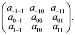
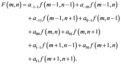
Filters mentioned above are called linear spatial filters. Their application to a digital image creates a new image using a linear combination of brightness values in the surrounding pixels. The intensities of the digital image in each pixel are defined by the matrix . If we want to apply a filter comprising eight neighboring pixels with different weights, we construct the
 ![]() weights matrix
weights matrix
New digital image has the intensity in each pixel given by a matrix  and their values are
This corresponds to the sum of all the values of the ![]() matrix we get as a pointwise multiplication of the filter
matrix we get as a pointwise multiplication of the filter ![]() matrix cut around the filtered pixel. Mathematically, it is a discrete convolution
matrix cut around the filtered pixel. Mathematically, it is a discrete convolution

For defining the orbit convolutions we proceed in a similar way as for the discrete cosine transform DCT II, where for two functions  and
and ![]() it is defined
it is defined

and for cosine transform ![]() the following relation holds [3]
the following relation holds [3]

3. Weyl Group Orbit Functions
3.1. Weyl Groups and Affine Weyl Groups
We consider the simple Lie algebras of rank two, namely  and
and . Each of them is described by its set of simple roots
![]() . In the case of
. In the case of , the roots are of the same length, for
  and
and  we distinguish so-called short root and long root. We use the standard normalization
  for the long roots. Coroots are defined as
![]() . Moreover, we define the weights
. Moreover, we define the weights ![]() and coweights
and coweights , which are dual to root and coroots in the sense
 . The weight lattice
  is defined as all integer combinations of weights.
We denote the reflections with respect to the hyperplanes orthogonal to the simple roots by  and
and , i.e.,
 ![]() They generate a Weyl group corresponding to each Lie algebra. The action of
They generate a Weyl group corresponding to each Lie algebra. The action of ![]() on the set of simple roots gives a root system
on the set of simple roots gives a root system  in
in . It contains a unique highest root
 , where the coefficients
 ![]() are called the marks. Analogously, a root system
are called the marks. Analogously, a root system  is obtained from the action of
 ![]() on the set of coroots, its highest root is denoted by
on the set of coroots, its highest root is denoted by , the coefficients are called the dual marks.
Let  denote the reflection with respect to the hyperplane orthogonal to
  and we define
  by
by

The affine Weyl group  is generated by
 . Its fundamental domain is a connected subset of
  such that it contains exactly one point of each affine Weyl group orbit. It can be chosen [4] as the convex hull of the points
 . The root systems and the fundamental domains of affine Weyl group of
and  are depicted in Figure 1.
The even Weyl group  is defined as
 . Its fundamental domain is
![]() , where
, where  is a simple reflection and
  denotes the interior of
  [5]. Corresponding dual even affine Weyl group is denoted
  and its fundamental domain is given by
 .
.
3.2. Weyl Group Orbit Functions
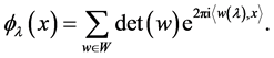
Three families of Weyl group orbit functions, so-called C-, Sand E-functions, are defined in the context of any Weyl group. Their complete description can be found in the series of papers [6-8]. The family of C-functions is defined as follows: For every  and
and ![]() we have
we have

The functions are invariant with respect to the affine Weyl group, therefore, we can consider ![]() only.
only.
The family of S-functions is defined for every  and
and ![]() as
as
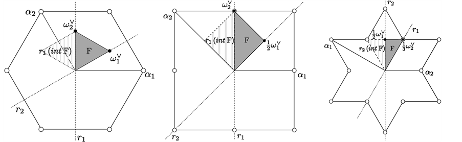
Figure 1. Root system of  and
and . Dots denotes the roots, dashed lines the hyperplanes orthogonal to the simple roots and the gray triangle is the fundamental domain of the corresponding affine Weyl group.
They are antiinvariant with respect to , moreover, they vanish on the boundary of the fundamental domain. We can consider
 .
.
Finally, the E-orbit functions are defined for every  and
and ![]() as
as

They are invariant with respect to the even affine Weyl group, we restrict them on .
.
For Weyl groups with two different lengths of root in their root system other families of orbit functions can be defined. For more details see [9,10]. In this paper, we consider convolution based on the Cand E-functions, S-functions do not differ significantly from the C-functions case.
3.3. Discrete Orthogonality and Orbit Transform
The method of discretization of orbit functions was described in detail in the papers [4,5]. The general idea is the following: In the fundamental domain we define a finite grid of points , where
  is an integer of our choice which allows us to control the density of the grid. A discrete scalar product of functions is then defined using this points. We describe a finite family of orbit functions which are pairwise orthogonal with respect to this scalar product by defining a grid of parameters labeling the functions. Finally, we give the explicit orthogonality relations. Appendix 1 summarize details about the choice of the grids.
We consider a space of discrete functions sampled on the points of  with a scalar product defined for each pair of functions
  as
as
 (1)
(1)
The weight function  is given by the order of the Weyl orbit of
 ,
, . The set of parameters
 ![]() gives us a finite family of orbit functions which are pairwise orthogonal with respect to the scalar product (1).
gives us a finite family of orbit functions which are pairwise orthogonal with respect to the scalar product (1).
For every  it holds that
 (2)
(2)
where the coefficient  is the order of the stabilizer of
![]() ,
,  is determinant of the Cartan matrix of the corresponding Weyl group and
  is its order. The values of
 ,
,  ,
,  and
and  are listed in Appendix 2.
The discrete orthogonality allows us to perform a Fourier like transform, called C-orbit transform. We consider a function  sampled on the points of
 . We can interpolate it by a sum of C-functions
 (3)
(3)
where we require  for every
 . Therefore, the coefficients
  are equal to
 (4)
(4)
In the case of E-orbit functions we consider the grids  and
and![]() . The scalar product is defined as
. The scalar product is defined as
 (5)
(5)
The weight function ![]() is given by the order of the even Weyl orbit of
is given by the order of the even Weyl orbit of ,
, .
.
For every  it holds that
 (6)
(6)
where the coefficient  is the order of the stabilizer of
 ![]() and
and  is the order of the even Weyl group.. The values of
 ,
, ![]() and
and  are listed in Appendix 2.
The E-orbit transform is provided as follows. We consider a function  sampled on the points of
 . We can interpolate it by a sum of E-functions
 (7)
(7)
where we require ![]() for every
for every . Therefore, the coefficients
  are equal to
 (8)
(8)
4. Orbit Convolution
4.1. Orbit Convolution Theorem
The main aim of this work is to define a discrete orbit functions convolution, i.e., a mapping of two functions sampled on  which respects a relation analogous to the classical convolution theorem. Such definition comes naturally from the orbit functions discretization theory.
The ![]() -orbit convolution is for every pair of discrete functions
-orbit convolution is for every pair of discrete functions  and
and  defined as
 (9)
(9)
Such a convolution is well defined, the shifts in the convolution kernel ![]() respect the symmetry of the Weyl group of
respect the symmetry of the Weyl group of . We can write the
 ![]() -orbit convolution theorem.
-orbit convolution theorem.
Theorem 1 Let  be any functions defined on the points of
  and
and . Then
 (10)
(10)
where  and
and  are the
 ![]() -orbit transforms of
-orbit transforms of  and
and ![]() given by (3).
given by (3).
Its proof is straightforward, it uses the relations (4) and the following formula for the product of an orbit function with the complex conjugate of an orbit function with the same label but different argument:
 (11)
(11)
Analogously, the  -orbit convolution is defined for discrete functions
  sampled on
  and
and  as
as
 (12)
(12)
The E-orbit convolution theorem is then the following.
Theorem 2 Let  be any functions defined on the points of
  and
and . Then
 (13)
(13)
where  and
and  are the
  -orbit transforms of
  and
and ![]() given by (7).
given by (7).
4.2. Examples of Image Filtering
For the purpose of demonstrating the differences between the orbit convolution and convolution on  we take an artificial image of a hexagon. Three of spatial filters are presented: a mean filter, often used for image noising; a sharpen filter which is useful for contrast enhancing; and a simple edge detecting filter which suppresses the monotonic (in the sense of pixel brightness) parts of an image.
In  these filters are described by matrices:

The filters are constructed to be as similar to the filters used for orbit convolution as possible. There are some restrictions for the orbit convolution coming from its definition, the most significant is the summation over all reflections of the convolution kernel. This property is unpleasant, since it does not give us the possibility to apply changes in a single direction, i.e., detecting only horizontal edges. For this reason we cannot use all convolution kernels we can use for image filtering in .
.
When developing a spatial filter for orbit convolution from kernel for filtering in  we have to take the formula (9) into account. Many filters are supposed to preserve the average value of brightness in the image. In the frequency domain the related value is situated in the point
 . The normalization of the filter is done by dividing the weighted sum of kernel points by coefficients
 . There is also a second level of normalization, arising from the summation over all Weyl reflections of a point, the filter is divided by the number of reflections. Some filters, mostly the ones based on differences, have the weighted sum equal to zero, thus not requiring any normalization.
There are two major restrictions for the orbit convolution kernels: the reflection of the kernel, which disables filtering in a single direction, and the placement of the kernel center. For the convolution on  the kernel center is located in the middle point of the kernel, for orbit convolution the center is in the point
 . This brings further restriction, the filter cannot count with all neighboring points.
Filters for orbit convolution are defined in the following way:

For the orbit convolution demonstration we used the hexagon image, see Figure 2, and filtered it via convolution on  and via C-orbit convolution on
  group to have a comparison for similar filters for both methods. The results are depicted on Figures 3-5.
The differences between the convolution on  and orbit convolution via C-orbit transform on
  group are very little. One of the reason is the inequality of convolution kernels for both types of convolution.
5. Conclusions
1) In the case of  and
and  orbit functions, there are 7 more families of orbit function defined, and the
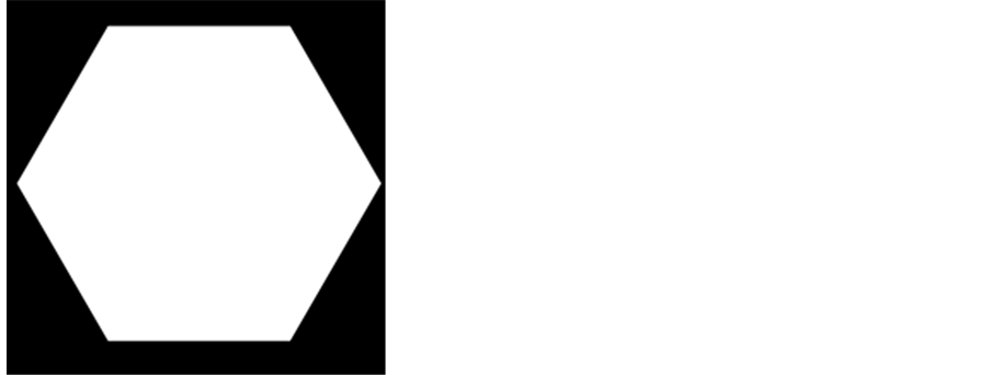
Figure 2. Original image, used for filtering.

Figure 3. Image filtered with blurring filter, via ![]() convolution (left) and orbit convolution (right).
convolution (left) and orbit convolution (right).

Figure 4. Sharpening previously blurred image, ![]() (left) and orbit (right) convolution.
(left) and orbit (right) convolution.
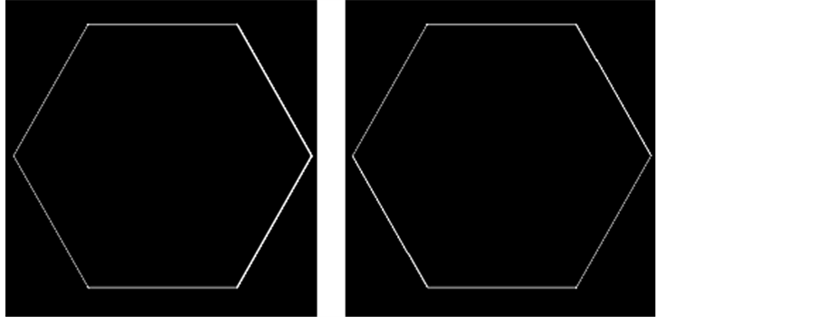
Figure 5. Edge detection in the original image, on the left with ![]() convolution, on the right with orbit one.
convolution, on the right with orbit one.
orbit convolution theorem can be formulated for each of them. This gives us bigger choice of the shape of the fundamental domain suitable for the image.
2) The method described here can be generalized to Weyl group of any rank. Therefore, it can be used for more general problems than the image processing.
3) The orbit convolution takes an advantage from the symmetry of the underlying Weyl group. On the other hand, as there is no fast algorithm yet, the computation takes more time than standard Fourier or cosine transform. One of our future projects is finding such a fast algorithm.
Acknowledgements
This work is supported by the European Union under the project Support of inter-sectoral mobility and quality enhancement of research teams at Czech Technical University in Prague CZ.1.07/2.3.00/30.0034.
REFERENCES
- R. C. Gonzalez and R. E. Woods, “Digital Image Processing,” Addison Wesley Longman, Inc., Reading, 1992.
- H. G. Granlund and H. Knutsson, “Signal Processing for Computer Vision,” Kluwer Academic Publisher, Dordrecht, 1995.
- N. X. Thao, V. A. Kakichev and V. K. Tuan, “On the Generalized Convolutions for Fourier Cosine and Sine Transforms” East-West Journal of Mathematics, Vol. 1, 1998, pp. 85-90.
- J. Hrivnák and J. Patera, “On Discretization of Tori of Compact Simple Lie Groups,” Journal of Physics A: Mathematical and Theoretical, Vol. 42, 2009, Article ID: 385208.
- J. Hrivnák and J. Patera, “On E-Discretization of Tori of Compact Simple Lie Groups,” Journal of Physics A: Mathematical and Theoretical, Vol. 43, No. 16, 2010, Article ID: 165206.
- A. Klimyk and J. Patera, “Orbit Functions,” SIGMA (Symmetry, Integrability and Geometry: Methods and Applications), Vol. 2, 2006, p. 6.
- A. Klimyk and J. Patera, “Antisymmetric Orbit Functions,” SIGMA (Symmetry, Integrability and Geometry: Methods and Applications), Vol. 3, 2007, 83 p.
- A. Klimyk and J. Patera, “E-Orbit Functions,” SIGMA (Symmetry, Integrability and Geometry: Methods and Applications), Vol. 4, 2008, 57 p.
- L. Háková, J. Hrivnák and J. Patera, “Six Types of E-Functions of the Lie Groups O(5) and G(2),” Journal of Physics A: Mathematical and Theoretical, Vol. 45, No. 12, 2012, Article ID: 125201.
- R. V. Moody, L. Motlochová and J. Patera, “New Families of Weyl Group Orbit Functions,” arXiv:1202.4.
Appendix
1. Grids FM and (M
In this Section we describe in detail the grids of points and grids of parameters used in the discretization of orbit functions [4,5].
We consider four lattices in . The root lattice
 ; the coroot lattice
  and their duals
  and
and  which are called the weight lattice and coweight lattice respectively.
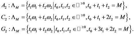
Two finite lattice grids depending on an integer parameter  are defined as follows: We consider the
 ![]()
invariant group  and we define the set of points
  as such cosets from
  which have a representative in
 . It can be written as

The explicit formulas are then obtain by using the marks  and
and  of the concrete group. Namely, the marks are
  for
for ,
,  for
for  and
and  for
for .
.
 (14)
(14)
For the grid of parameters we take the ![]() invariant group
invariant group  and we consider its cosets with a representative element in
 . Explicitly,

where the duals marks  and
and  are
are  for
for ,
,  for
for  and
and  for
for .
.
 (15)
(15)
The grids for the ![]() transform are defined analogously,
transform are defined analogously,

where ![]() and
and  for a simple reflection
 .
.
2. Values of  and
and 
We summarize values of all the constants and functions needed in formulas (2), (3), (6), (7).
The orders of the corresponding Weyl groups and even Weyl groups are:
 (16)
(16)
The determinants of the corresponding Cartan matrix are:
 (17)
(17)
The values of  and
and  are listed in Tables 1 and 2.
Let  be in
be in . For
. For  it holds that
 . The values of
 ![]() for
for ![]() are listed in Table3
are listed in Table3
Let ![]() be in
be in . For
. For  it holds that
 . The other values of
  are listed in Table4

Table 1. The coefficients  of
of ,
,  and
and . The variables
 ,
,  , are nonnegative integers and have the same meaning as in (14).
Table 2. The coefficients  of
of ,
,  and
and . The variables
 ,
,  , are nonnegative integers and have the same meaning as in (15).
Table 3. The coefficients  of
of ,
,  and
and . The variables
 ,
,  , are nonnegative integers and have the same meaning as in (14).
Table 4. The coefficients  of
of ,
,  and
and . The variables
 ,
,  , are nonnegative integers and have the same meaning as in (15).