ABSTRACT

A new algorithm is presented for solving Troesch’s problem. The numerical scheme based on the sinc-collocation technique is deduced. The equation is reduced to systems of nonlinear algebraic equations. Some numerical experiments are made. Compared with the modified homotopy perturbation technique (MHP), the variational iteration method and the Adomian decomposition method. It is shown that the sinc-collocation method yields better results.

1. Introduction

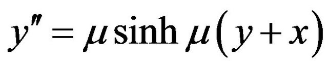
In this paper, we consider a two-point boundary value problem, Troesch’s problem [1-3], defined by

(1)

(2)

where is a positive constant. This problem arises in an investigation of the confinement of a plasma column by radiation pressure [4] and also in the theory of gas porous electrodes [5,6]. This problem has been studied extensively. Troesch found its numerical solution in [7] using the shooting method, in [8] using the decomposition technique, in [9-11] using the variational iteration method, in [12] using a combination of the multipoint shooting method with the continuation and perturbation technique, in [13] using the quasilinearization method, in [14] using the method of transformation groups, in [15] the invariant imbedding method, in [16] using the inverse shooting method, in [17] using the modified homotopy perturbation method, in [18] using sinc-Galerkin method, in [19] using B-spline method, in [20] using the differential transform method and in [21] using chebychev collocation method.

The purpose of this paper is to introduce a novel approach based on sinc function for the numerical solution of the class of nonlinear boundary value problems given in (1)-(2). Sinc approximation have become increasingly important in numerical analysis. Most commonly used techniques with sinc-collocation have been examined in [22-24] and references therein. The error of the method converges to zero like, as, where N is the numerical of collocation points used, and where k is a positive constant independent of N.

The aim of this work is two folds. First we aim to investigate the ODEs of a variety of distinct orders, linear or nonlinear, to show that sinc-collocation method can work as a unified method. Second we aim to confirm the power of the sinc-collocation method in handling scientific and engineering problems.

The remaining structure of this article is organized as follows: a brief introduction to the sinc function is presented in Section 2. In Section 3, the sinc-collocation approach for the solution of Troesch’s problem is described. The results are compared with the exact solutions and some existing numerical solutions in Section 4. Finally, in Section 5, a conclusion is given that briefly summarizes the results.

2. Sinc Function

A general review of sinc function approximation is given in [25,26] and the recent papers [27-29]. Hence, only properties important to the present goals are outlined in this section.

If is defined on the real line, then for the Whittaker cardinal expansion of f

where, and the mesh size is given by

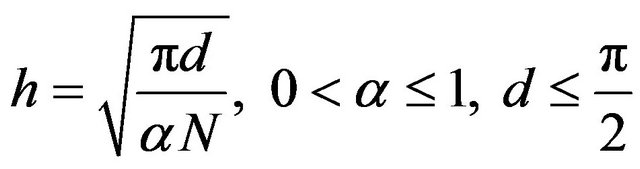(3)

where N is suitably chosen and depends on the asymptotic behavior of. The basis functions on are then given by

and

(4)

The interpolation formula for over takes the form

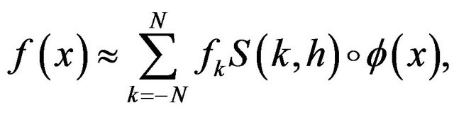(5)

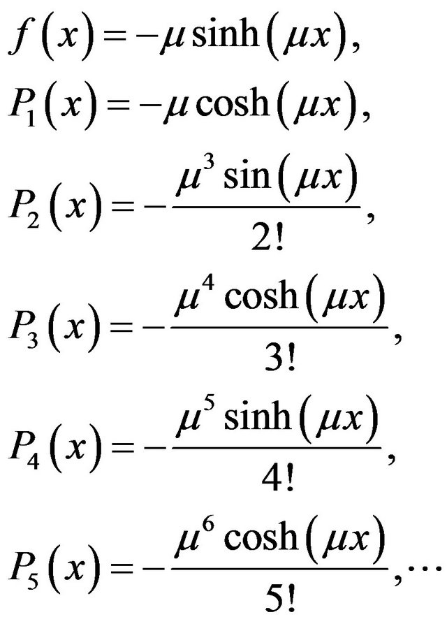
The n-th derivative of the function at points can be approximated using a finite number of terms as

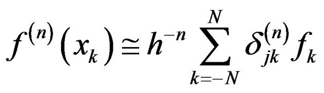(6)

where

The quadrature formula of is given by

(7)

We consider the following definitions and theorems in [26].

Definition 1.

Let be a simply-connected domain in the complex plane having boundary. Let and denote two distinct points of and denote a conformal map of onto, where denote the region

such that and. Let denote the inverse map, and let be defined by

Given and a positive number let us set, let us also by.

Definition 2.

Let be the set of all analytic functions, for which there exists a constant, such that

Theorem 1.

Let, let be a positive integer, and be selected by the Formula (3) then there exist positive constant, independent of, such that

.

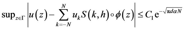3. The Description of Sinc-Collocation Scheme

First, the sinc function composed with various conformal mappings, , are zero at the endpoints of the interval. Since the boundary conditions are nonhomogeneous, then these conditions need be converted to homogeneous ones via an interpolation by a known function. The nonhomogeneous boundary conditions in (2) can be transformed to homogeneous boundary conditions by the change of dependent variable. The new problem with homogeneous boundary conditions is then

(8)

subject to the boundary conditions

(9)

To obtain its approximate solution of Equations (8) and (9), we expand around

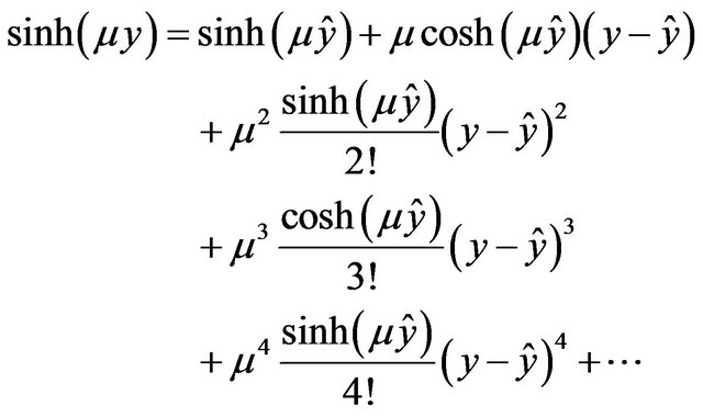
Particularly, if, then

and

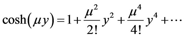
The Equation (8) becomes

(10)

where

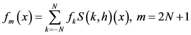
The approximate solution for is represented by the formula

(11)

We need the following lemma.

Lemma.

The following relation holds

(12)

where N and are now dependent on both and.

Replacing the terms of (10) with the appropriate representation defined in (5), (6), and (12) and applying the collocation to it, we eventually obtain the following theorem.

Theorem 2.

If the assumed approximate solution of problem (10) and (9) is (11), then the discrete sinc-collocation system for the determination of the unknown coefficients is given by

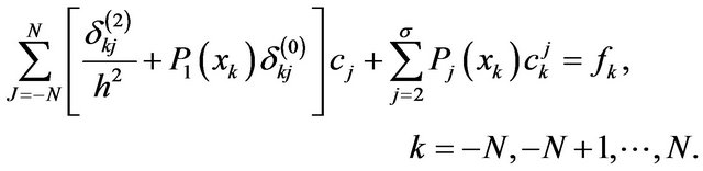(13)

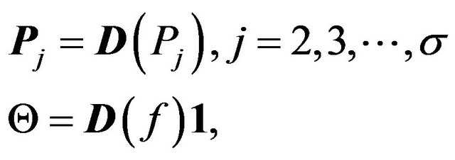
The following notation will be necessary for writing down the system. Let be the diagonal matrix

(14)

and define the matrices (see [30]) for by

(15)

whose kj-th entry is given by

Let c be the m-vector with j-th component given by, let be the m-vector with j-th component given by, and 1 is an m-vector each of whose components is 1. In this notation the system in (13) takes the matrix form

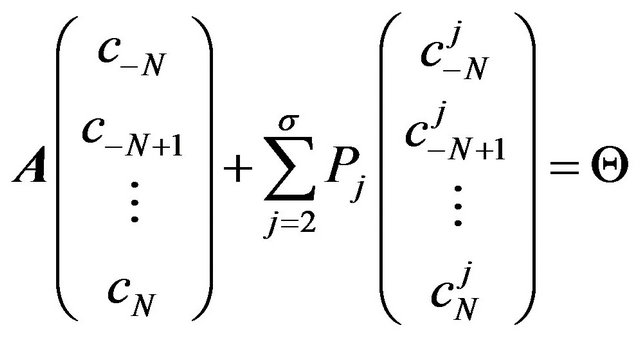(16)

where

and

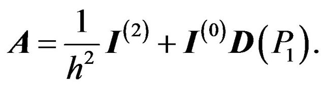
Now we have a nonlinear system of equation of the m unknown coefficients, namely,.

We can obtain the coefficient of the approximate solution by solving this nonlinear system by Newton’s method. The solution gives the coefficients in the approximate sinc-collocation solution of. Then, the approximate solution of (1) is

Newton’s Method.

To solve the system of Equation (16), we express these equations as the simultaneous zeroing of a set of functions, where the number of functions to be zeroed is equal to the number of independent variables.

(17)

A very important method for the solution of Equation (17) is Newton’s method:

Let be the guess at the solution for iteration i. Assuming the is not small enough, we seek an update vectors

i.e.

(18)

such that. Using the multidimensional extension of Taylor’s theorem to approximate the variation of in the neighborhood of gives

(19)

where is the Jacobian of the system of equations:

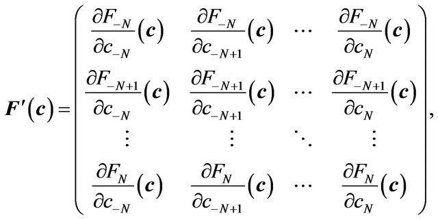(20)

Neglecting higher order terms and designating as the Jacobian evaluated at. We can rearrange Equation (19)

(21)

The goal of Newton iterations is to make , so setting that term to zero in the preceding equation gives

(22)

Equation (22) is a system of m linear equations in the m unknown. Each Newton iteration step involves evaluation of the vector, the matrix and the solution to Equation (22). A common numerical practice is to stop the Newton iteration whenever the distance between two iterates is less than a given tolerance, i.e. when

• Algorithm.

• Initialize:

• For

•

• If is small enough, stop

• Compute

• Solve

•

• End.

4. Numerical Examples

The closed form solution to this problem in terms of the Jacobian elliptic function has been given [3] as

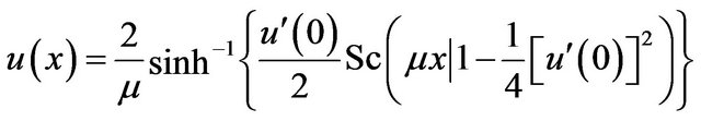(23)

where, the derivative of at 0, is given by the expression, with being the solution of the transcendental equation

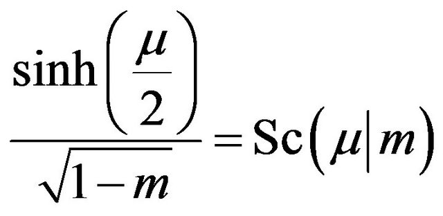
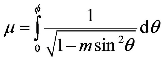
where the Jacobian elliptic function [2,31] is defined by 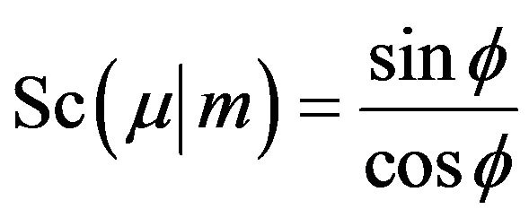where and are related by the integral

In Tables 1 and 2 the numerical solution obtained by sinc-collocation method is compared with the exact solution derived from Equation (23) and with the numerical solution obtained by the modified homotopy perturbation technique (MHP) [17], variation method [9] and decomposition method [8] for the case and respectively .

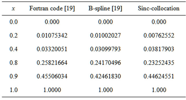
In Table 3, the numerical solution obtained by the sinc-collocation method for is compared with the numerical approximation of the exact solutions given by a Fortran code called TWPBVP and the numerical solution obtained by B-spline collocation method [19].

5. Discussions

There are two main goals that we aimed for this work. The first is to employ the powerful sinc-collocation method to investigate nonlinear ordinary differential equations. The second is to show the power of this method and its significant features. The two goals are achieved.

In [27], we compared the performance of the collocation and Galerkin methods using sinc bases for solving linear and nonlinear second order two-point boundary value problems and shown that the most significant virtue

Table 1. Numerical solutions of Troesch’s problem for the case μ = 0.5.

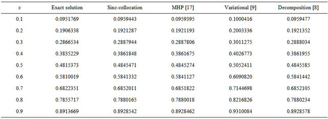
Table 2. Numerical solutions of Troesch’s problem for the case μ = 1.

Table 3. Numerical solutions of Troesch’s problem for the case μ = 5.

of the collocation procedure is its ease in application. The collocation method easily generalizes to problems having general boundary conditions.

REFERENCES

- M. Abramowitz and I. Stegun, “Handbook of Mathematical Functions,” Dover, New York, 1972.
- A. Erdelyi, W. Magnus, F. Oberhettinger and F. Tricomi, “Higher Transcendental Functions,” Vol. 2, McGraw-Hill, New York, 1953.
- S. Roberts and J. Shipman, “On the Closed form Solution of Troesch’s Problem,” Journal of Computational Physics, Vol. 21, No. 3, 1976, pp. 291-304. doi:10.1016/0021-9991(76)90026-7
- E. Weibel, “On the Confinement of a Plasma by Magnetostatic Fields,” Physics of Fluids, Vol. 2, No. 1, 1959, pp. 52-56. doi:10.1063/1.1724391
- D. Gidaspow and B. Baker, “A Model for Discharge of Storage Batteries,” Journal of the Electrochemical Society, Vol. 120, No. 8, 1973, pp. 1005-1010. doi:10.1149/1.2403617
- V. Markin, A. Chernenko, Y. Chizmadehev and Y. Chirkov, “Aspects of the Theory of Gas Porous Electrodes,” In: V. S. Bagotskii and Y. B. Vasilev, Eds., Fuel Cells: Their Electrochemical Kinetics, Consultants Bureau, New York, 1966, pp. 21-33.
- B. A. Troesch, “A Simple Approach to a Sensitive TwoPoint Boundary Value Problem,” Journal of Computational Physics, Vol. 21, No. 3, 1976, pp. 279-290. doi:10.1016/0021-9991(76)90025-5
- E. Deeba, S. Khuri and S. Xie, “An Algorithm for Solving Boundary Value Problems,” Journal of Computational Physics, Vol. 159, No. 2, 2000, pp. 125-138. doi:10.1006/jcph.2000.6452
- S. Chang, “A Variational Iteration Method for Solving Troesch’s Problem,” Journal of Computational and Applied Mathematics, Vol. 234, No. 10, 2010, pp. 3043- 3047. doi:10.1016/j.cam.2010.04.018
- S. A. Khuri, “A Numerical Algorithm for Solving Troesch’s Problem,” International Journal of Computer Mathematics, Vol. 80, No. 4, 2003, pp. 493-498. doi:10.1080/0020716022000009228
- S. Momani, S. Abuasad and Z. Odibat, “Variational Iteration Method for Solving Nonlinear Boundary Value Problems,” Applied Mathematics and Computation, Vol. 183, No. 2, 2006, pp. 1351-1358. doi:10.1016/j.amc.2006.05.138
- S. Roberts and J. Shipman, “Solution of Troesch’s TwoPoint Boundary Value Problem by a Combination of Techniques,” Journal of Computational Physics, Vol. 10, No. 2, 1972, pp. 232-241. doi:10.1016/0021-9991(72)90063-0
- A. Miele, A. Agarwal and J. Tietze, “Solution of TwoPoint Boundary-Value Problems with Jacobian Matrix Characterized by Large Positive Eigenvalues,” Journal of Computational Physics, Vol. 15, No. 2, 1974, pp. 117- 133. doi:10.1016/0021-9991(74)90080-1
- J. Chiou and T. Na, “On the Solution of Troesch’s Nonlinear Two-Point Boundary Value Problem Using an Initial Value Method,” Journal of Computational Physics, Vol. 19, No. 3, 1975, pp. 311-316. doi:10.1016/0021-9991(75)90080-7
- M. Scott, “On the Conversion of Boundary-Value Problems into Stable Initial-Value Problems via Several Invariant Imbedding Algorithms,” In: A. K. Aziz, Ed., Numerical Solutions of Boundary-Value Problems for Ordinary Differential Equations, Academic Press, New York, 1975, pp. 89-146.
- J. Snyman, “Continuous and Discontinuous Numerical Solutions to the Troesch Problem,” Journal of Computational and Applied Mathematics, Vol. 5, No. 3, 1979, pp. 171-175. doi:10.1016/0377-0427(79)90002-5
- X. Feng, L. Mei and G. He, “An Efficient Algorithm for Solving Troesch’s Problem,” Applied Mathematics and Computation, Vol. 189, No. 1, 2007, pp. 500-507. doi:10.1016/j.amc.2006.11.161
- M. Zarebnia and M. Sajjadian, “The Sinc-Galerkin Method for Solving Troesch’s Problem,” Mathematical and Computer Modelling, Vol. 56, No. 9-10, 2012, pp. 218- 228. doi:10.1016/j.mcm.2011.11.071
- S. Khuri and A. Sayfy, “Troesch’s Problem: A B-Spline Collocation Approach,” Mathematical and Computer Modelling, Vol. 54, No. 9-10, 2011, pp. 1907-1918. doi:10.1016/j.mcm.2011.04.030
- S. Chang and I. Chang, “A New Algorithm for Calculating One-Dimensional Differential Transform of Nonlinear Functions,” Applied Mathematics and Computation, Vol. 195, No. 2, 2008, pp. 799-808. doi:10.1016/j.amc.2007.05.026
- M. El-Gamel and M. Sameeh, “A Chebychev Collocation Method for Solving Troesch’s Problem,” International Journal of Mathematics and Computer Applications Research, Vol. 3, No. 2, 2013, pp. 23-32.
- B. Bialecki, “Sinc-Collocation Methods for Two-Point Boundary Value Problems,” IMA Journal of Numerial Analysis, Vol. 11, No. 3, 1991, pp. 357-375. doi:10.1093/imanum/11.3.357
- M. Muhammad, A. Nurmuhammada, M. Moria and M. Sugiharab, “Numerical Solution of Integral Equations by Means of the Sinc-Collocation Method Based on the Double Exponential Transformation,” Journal of Computational and Applied Mathematics, Vol. 177, No. 2, 2005, pp. 269-286. doi:10.1016/j.cam.2004.09.019
- A. Mohsen and M. El-Gamel, “A Sinc-Collocation Method for the Linear Fredholm Integro-Differential Equations,” Zeitschrift für Angewandte Mathematik und Physik, Vol. 58, No. 3, 2007, pp. 380-390. doi:10.1007/s00033-006-5124-5
- J. Lund and K. Bowers, “Sinc Methods for Quadrature and Differential Equations,” SIAM, Philadelphia, 1992. doi:10.1137/1.9781611971637
- F. Stenger, “Numerical Methods Based on Sinc and Analytic Functions,” Springer, New York, 1993. doi:10.1007/978-1-4612-2706-9
- A. Mohsen and M. El-Gamel, “On the Galerkin and Collocation Methods for Two-Point Boundary Value Problems Using Sinc Bases,” Computers & Mathematics with Applications, Vol. 56, No. 4, 2008, pp. 930-941. doi:10.1016/j.camwa.2008.01.023
- A. Mohsen and M. El-Gamel, “On the Numerical Solution of Linear and Nonlinear Volterra Integral and Integro-Differential Equations,” Applied Mathematics and Computation, Vol. 217, No. 7, 2010, pp. 3330-3337. doi:10.1016/j.amc.2010.08.065
- M. El-Gamel, “Sinc-Collocation Method for Solving Linear and Nonlinear System of Second-Order Boundary Value Problems,” Applied Mathematics, Vol. 3, No 11, 2012, pp. 1627-1633. doi:10.4236/am.2012.311225
- V. Grenander and G. Szego, “Toeplitz Forms and Their Applications,” 2nd Edition, Chelsea Publishing Co., Orlando, 1985.