Applied Mathematics
Vol.3 No.10A(2012), Article ID:24114,12 pages DOI:10.4236/am.2012.330193
Robust Optimum Design of Thrust Hydrodynamic Bearings for Hard Disk Drives
Department of Mechanical Engineering, Tokai University, Hiratsuka, Japan
Email: hiromu@keyaki.cc.u-tokai.ac.jp, 0btad005@mail.tokai-u.jp
Received July 4, 2012; revised August 4, 2012; accepted August 11, 2012
Keywords: Robust Optimum Design; Hard Disk Drive; Hydrodynamic Bearing; Tolerance; Statistical Method
ABSTRACT
This paper describes the robust optimum design which combines the geometrical optimization method proposed by Hashimoto and statistical method. Recently, 2.5″ hard disk drives (HDDs) are widely used for mobile devices such as laptops, video cameras and car navigation systems. In mobile applications, high durability towards external vibrations and shocks are essentials to the bearings of HDD spindle motor. In addition, the bearing characteristics are influenced by manufacturing error because of small size of the bearings of HDD. In this paper, the geometrical optimization is carried out to maximize the bearing stiffness using sequential quadratic programming to improve vibration characteristics. Additionally, the bearing stiffness is analyzed considering dimensional tolerance of the bearing using statistical method. The dimensional tolerance is assumed to distribute according to the Gaussian distribution, and then the bearing stiffness is estimated by combining the expectation and standard deviation. As a result, in the robust optimum design, new groove geometry of bearing can be obtained in which the bearing stiffness is four times higher than the stiffness of conventional spiral groove bearing. Moreover, the bearing has lower variability compared with the result of optimum design neglecting dimensional tolerance.
1. Introduction
Recently, demand of hard disk drives (HDDs) has been continued to expand because of development of information technology in industries. Especially, 2.5″ HDDs are widely used for many information devices such as laptops, digital video cameras and car navigation systems. Consequently, convenience and performance of information devices have been improving year by year. In the meantime, usage environments in which HDDs are used under the conditions occurring vibrations have been being severe than before. Therefore, improvement of vibration characteristics of HDDs has been strongly demanded. Hydrodynamic bearings, which are used in spindle motor of HDDs, are one of key machine elements to improve vibration characteristics of HDDs. The hydrodynamic bearings which mainly have grooves called the spiral or herring-bone groove are traditionally used for HDDs spindle motor. There are several researchers [1-7] who attempted to investigate the research related to the improvement of vibration characteristics of the hydrodynamic bearings. However, they are still insufficient for a significant improvement of bearing characteristics. One reason is because the groove geometry is fixed on the spiral or herring-bone grooves. On the other hand, Hashimoto and Ochiai [8] dealt with the geometrical optimization aimed at discovering the optimum groove geometry which have never found before and improving dramatically bearing stiffness of thrust air bearings. In addition, the higher performance of the bearing having optimum groove geometry is experimentally verified. Moreover, Ibrahim et al. [9] applied the same method of the geometrical optimization to thrust air bearings on HDD spindle motor and the effectiveness was theoretically discussed.
In the process of manufacturing thrust hydrodynamic bearings for 2.5″ HDDs, it is compulsory to maintain high dimensional accuracy due to high influence by manufacturing errors towards the bearing characteristics. Therefore, it is necessary to severely design considering the dimensional tolerance of design variables of the bearings. In that case, a new designing method which treats the tolerance numerically in advance is reasonable compared with the conventional method which determines the tolerance by trial-and-error method. In the conventional designing method of the bearings, a deterministic method neglecting the dimensional tolerance of design variables is being mainly used. For that reason, there are several researchers [10-14] who attempted to investigate the influence of manufacturing errors on the bearing characteristics through sensitivity analysis. However, as far as the authors know, there is no research which had carried out the optimum design with the consideration of manufacturing errors for the hydrodynamic bearings of HDD spindle motors. In this paper, the influence of dimensional tolerance on bearing characteristics is conducted using the statistical method. And then, the robust optimum design based on the geometrical optimization combined with the statistical method [15] is applied to thrust hydrodynamic bearings of 2.5″ HDD spindle motor. The results obtained are compared with the result by the conventional optimum design neglecting tolerance to verify the effectiveness of the proposed method.
2. Geometrical Optimization and Analysis of Bearing Characteristics
2.1. Geometrical Optimization
In this paper, the geometrical optimization proposed by Hashimoto and Ochiai [8] is applied to thrust hydrodynamic bearings for 2.5″ HDD spindle motor to drastically improve the bearing stiffness. In the process of optimizing the groove geometry, the initial geometry is established and a groove shape, which is likely to provide a maximal bearing stiffness, is determined by using the method of successive evolution from the initial geometry as shown in Figure 1. Therefore, spiral groove bearings are considered as the initial geometry to raise calculation efficiency because the spiral groove bearings have relatively high bearing stiffness compared with other types of bearings. The initial spiral groove geometries are flexibly modified using the cubic spline interpolation function as shown in Appendix I. The whole groove is partitioned into n parts in the r direction, and then each nodal point 
 is provided to the intersection with the cubic spline interpolation function. At the time when a groove geometry is gradually evolved
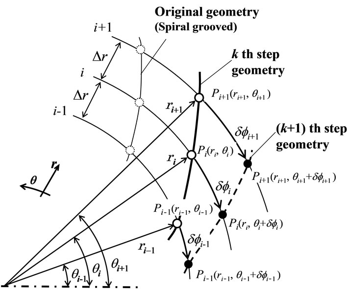
Figure 1. Method of changing groove boundary geometry.
from the previous stage (k step) to the present stage (k + 1 step) shown by the broken line in Figure 1, the r coordinate of each nodal point  is fixed, and the θ coordinate is changed when the angle δf moves in the positive direction or negative direction, resulting to a new nodal point
 . Then, the groove geometry is revised, using the new coordinate value that can be obtained using this way, and gradually evolved until the value of the bearing stiffness becomes maximum.
2.2. Analysis of Bearing Characteristics
In this paper, the calculation method of bearing characteristics is derived by applying the boundary-fitted coordinate system to adjust the geometrical optimization method. Moreover, in the process of analyzing the static and dynamic characteristics of the bearings, the perturbation method is applied to the Reynolds equivalent equation. The Reynolds equivalent equation can be solved by using the Newton-Raphson iteration method, and the static component p0 and dynamic component pt of pressure are obtained. These detailed calculation method is shown in Appendix II.
The load-carrying capacity W is obtained by the following integration:
 (1)
(1)
where pa indicates the atmospheric pressure.
The minimum oil lubricating film thickness hrmin is simultaneously determined from the equilibrium condition between the axial load acting on a thrust bearing and the bearing load-carrying capacity. The minimum oil lubricating film thickness hrmin is obtained by solving the following force balance equation:
 (2)
(2)
The spring coefficient k and damping coefficient c can be obtained, respectively, by integrating the real and imaginary parts of the dynamic pressure components, pt, as follows:
 (3)
(3)
 (4)
(4)
Finally, the bearing stiffness is given by the following equation.
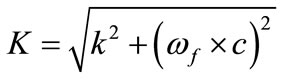 (5)
(5)
3. Estimation of Variability Using Statistical Method
Designing of the bearings for HDD spindle motor is required the high bearing performance and quality. Therefore, in this case, the optimum design is applied to the bearings for obtaining high bearing performance. On the other hand, bearing performance is highly influenced by manufacturing error because of small size of the bearings of HDD. However, the conventional method of designing the bearings was conducted using deterministic method, which neglected the dimensional tolerance. Hence, considering the influence of dimensional tolerance under product design is very important in terms of the quality and productivity of HDD spindle motors.
Figure 2 shows a conceptual diagram between design variables and variability of bearing performance. The vertical axis shows the typical bearing performance and the horizontal axis shows the typical design variables, for example, groove depth, groove width ratio and so on. As can be seen in the figure, variability of bearing performance shows non-uniform under the same range of dimensional tolerance. In the conventional optimum design neglecting tolerance, solution A can be obtained as optimized solution. Solution A is maximum value of bearing performance, but the variability becomes large when design variable is changed due to manufacturing error. On the other hand, variability of bearing performance of solution B is lower than that of solution A, although the bearing performance of solution A is better than solution B. That means, solution B has larger robustness of bearing performance compared with solution A. Therefore, it is necessary to find the design variable which can be obtained low variability with high bearing performance like solution B.
Figure 3 shows the relationship between bearing performance and variability. The figure shows the trade-off correlation between an increase of the variability and the bearing performance. In addition, it is possible that the spatial distribution of bearing performance is a multimodal distribution because the hydrodynamic bearings have
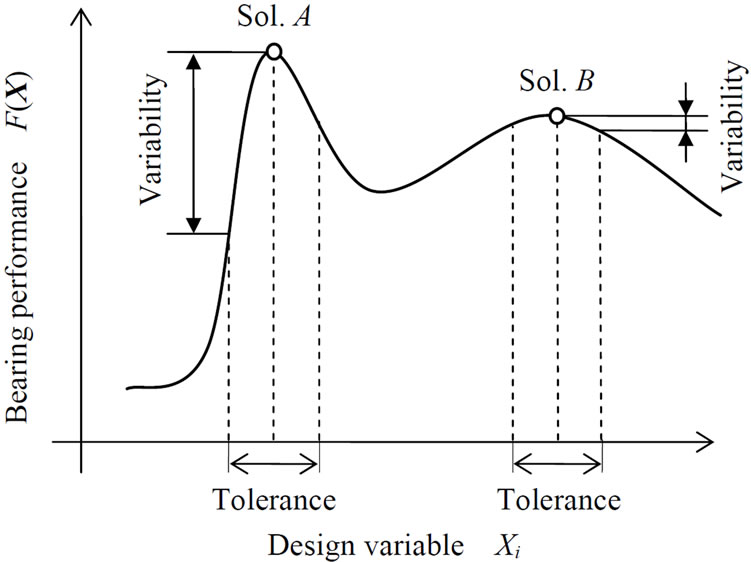
Figure 2. Variability of design variable and bearing performance.
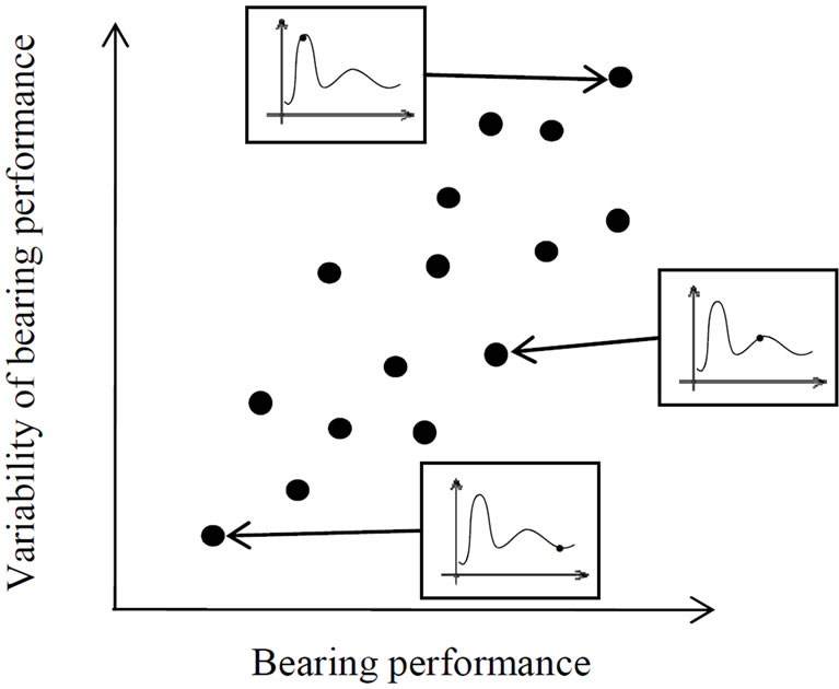
Figure 3. Trade-off correlation between bearing performance and variability of bearing performance.
relatively a lot of dimensions. In this case, it is important to treat multi-objective problem to obtain high bearing performance and robustness. Moreover, optimum design is needed to consider a statistical factor for designing of commercial HDDs. In this paper, the robust optimum design with high robustness is newly introduced to thrust hydrodynamic bearings. The evaluation method for the variability of the bearing performance using the statisticcal method is described as follows.
The variability of design variables is expressed by the probability density function, and then the robustness is estimated based on the expectation and standard deviation.
In the robust optimum design of thrust hydrodynamic bearings, the design variables such as groove depth and groove width ratio are given by the following expression as the random variable vector s.
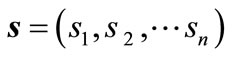 (6)
(6)
Figure 4 shows a conceptual diagram considering random variables s1 and s2. In the figure, a target value μi (i = 1 ~ n, where n represents the number of random variable) is the central value of the distribution of design variable, in which the design variable is assumed to distribute according to the Gaussian distribution within the range of ±Δsi from the central value μi. Consequently, the marginal probability density function for the component si of random variable vector s can be expressed as follows.
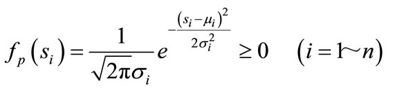 (7)
(7)
In this paper, the tolerance of the bearing dimension is considered as ±3σi.
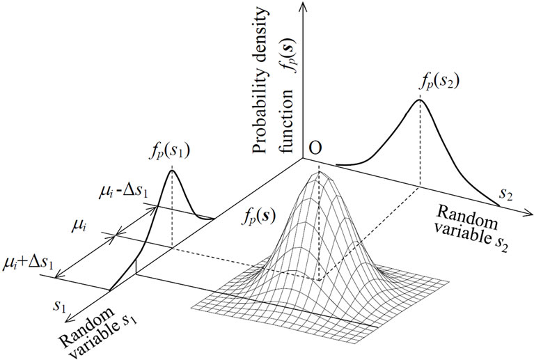
Figure 4. Probability density function.
When the marginal probability density functions of s are independent each other, the conjunctive probability density function is expressed as follows.
 (8)
(8)
As can be seen in Figure 4, when the variability is given to the design variables by the Gaussian distribution, the bearing performance will be distributed at the same time. Therefore, in estimating the bearing performance, it is necessary to use the expectation and standard deviation. The expectation and standard deviation of bearing performance are obtained, respectively, as follows,
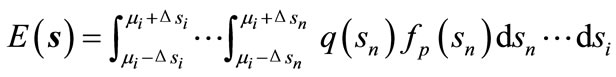 (9)
(9)
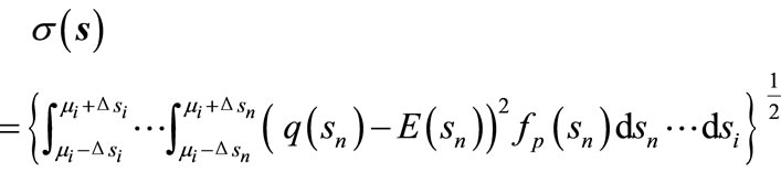 (10)
(10)
where q(si) indicates the bearing characteristics.
4. Robust Optimum Design of HDDs Considering Dimensional Tolerance
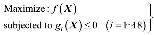
In this paper, the optimum problem is defined as maximizing the bearing stiffness of thrust hydrodynamic bearings to improve vibration characteristic of HDDs.
Figure 5 shows a schematic diagram of a 2.5″ HDD spindle motor with hydrodynamic bearings. A rotor which consists of a shaft, a hub, and two disks is supported by two thrust hydrodynamic bearings in the axial direction. In designing the bearings, we fixed the following design variables, in which outside radius of bearing r1 is 2.55 mm, inside radius of bearing r2 is 1.25 mm, rotational speed of shaft ns is 4200 rpm, seal ratio  is 0.636, inflow angle β is 15 deg., rotor mass m is 18.6 g and oil lubricant viscosity μ is 1.308 × 10⁻² Pa·s. The values are defined by referring specifications of an actual 2.5″ HDDs.

Figure 5. Schematic diagram of spindle motor of 2.5″ HDD and hydrodynamic thrust bearing, (1) Overall view of spindle motor, (2) Spiral grooved thrust bearing; (a) Position of thrust bearings and (b) Groove geometry.
In the present study, realizing an optimal design is first done by examining the magnitude of the bearing stiffness by changing the number of partitions of the cubic spline interpolation function in the r direction from two to six to process the optimal number of partitions. As a result, because the maximum value of the bearing stiffness is found when there are four partitions, the number of partitions in the r direction is fixed to four. In addition, groove depth hg, groove width ratio α and number of grooves N are given as design variables. Consequently, The design variable vector X consisting of the bearing dimensions is defined as follows:
 (11)
(11)
where f1 − f4 are extents of angle change from the initial geometry.
In the robust optimum design, the dimensional tolerance of design variables is considered. In this case, it is essential to consider the tolerance for all design variables. However, there is a possibility that computational time will be enormously large because of relatively large number of design variables. Therefore, the bearing dimensions with high sensitivity on the bearing performance are checked through the sensitivity analysis. As a result of the sensitivity analysis, groove depth hg and groove width ratio α have high sensitivity to the bearing characteristics, which are the bearing stiffness K and oil lubricating film thickness hr. Consequently, the dimensional tolerances of groove depth hg and groove width ratio α should be considered. In this paper, we determined experimentally the tolerance ranges of groove depth of Δhg = ±0.5, ±1.0, ±1.5, ±2.0 μm and groove width ratio of Δα = ±0.03, ±0.05.
On the other hand, as for the constraint functions, the upper and lower limits of the design variables in Equation (11) are considered. In addition, the allowable oil lubricating film thickness ha and non-negative damping coefficients c within variability are also considered as the constraints to guarantee the safety operation of the bearing. Moreover, the minimum groove width Lmin of grooved part as shown in Figure 6 is considered because there are some cases where the groove geometry will be in irregular shapes. The minimum groove width Lmin should be larger than the diameter of the industrial tool da. Then, in this paper, the diameter of industrial tool of da = 0.10 mm is determined with reference to prove diameter of industrial tool for an actual 2.5″ HDD spindle motor. The values of constraint conditions are shown in Table 1.
In the robust optimum design, it is necessary to reduce the variability of bearing characteristic value. Therefore, in this paper, the value of the standard deviation of bearing characteristic value obtained by Equation (10) including 3σ (F(X)) has to be less than 20% of the expectation value obtained by Equation (9). Then, the constraint equation is defined as follows,
 (12)
(12)
All of the constraint conditions are summarized as the following inequality expression:
 (13)
(13)
where the constraint functions in Equation (13) are defined as follows.
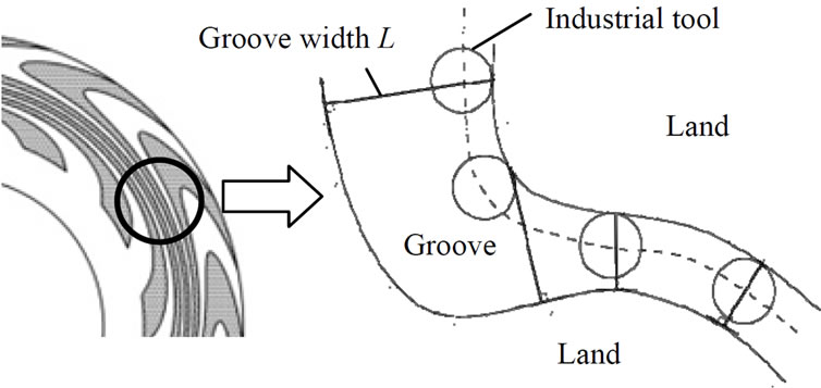
Figure 6. Relationship between groove width and diameter of industrial tool.
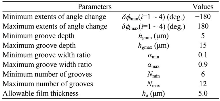
Table 1. Constraint conditions.
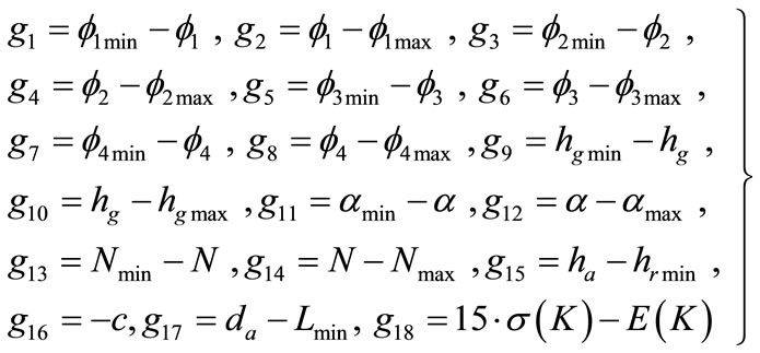 (14)
(14)
The objective function is expressed as follows:
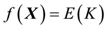 (15)
(15)
The optimum design problem of thrust hydrodynamic bearings is formulated from the above equation as follows:
 (16)
(16)
This optimum design problem is a typical nonlinear optimum design problem because the objective function and constraint functions are nonlinear including seven design variables. Therefore, the objective function has complicated multidimensional distribution. Consequently, at first several solutions are investigated through parametric study to find some local optimum solutions. Then, only the global optimum solution will be calculated using sequential quadratic programming (SQP) [8].
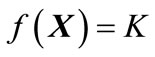
To clarify the validity of present robust optimum design, the results of the robust optimum design are compared with the results neglecting tolerance. Figures 7 and 8 show the flowcharts of the present robust optimum design and the conventional optimum design neglecting tolerance, respectively. As shown in these figures, the process of obtaining the values of the expectation and standard deviation neglecting tolerance are different from that of the robust optimum design. The calculation method of these values is described as follows.
In the optimum design neglecting tolerance, the same design variables and prescribed values used for the robust optimum design are given. However, the constraint condition of variability in Equation (12) and minimum groove width Lmin are excluded. Moreover, the objective function neglecting tolerance is different from the function of the robust optimum design because the dimensional tolerance is neglected. The objective function is defined as follows.
 (18)
(18)
The flow of the optimum design neglecting tolerance is shown in the range enclosed with single dotted line in Figure 8. The values of the expectation and standard deviation are calculated using the same tolerances of groove depth Δhg and groove width ratio Δα by Equations (9) and (10).
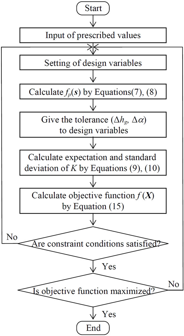
Figure 7. Flowchart of present robust optimum design.
5. Example of Optimized Results and Discussions
Figure 9 shows the results of groove geometries and static pressure distributions, respectively. In the figures, the groups (1) and (2) show respectively the results obtained by the robust optimum design (tolerance range, Δhg= ±1.0 μm, Δα = ±0.05) and by the optimum design neglecting tolerance and the group (3) shows the result of spiral groove bearing. The optimized groove bearings by the robust optimum design and by the optimum design neglecting tolerance as shown in Figures 9(1) and (2) have new groove geometries with similar geometry of spiral groove bearing in the inner vicinity; with an opposite spiral geometry in the outer vicinity. In this paper, such types of bearings that have an outer vicinity bends are called modified spiral groove bearing.
Table 2 shows the example of optimized results. As can be seen in Table 2, the values of bearing stiffness of modified spiral groove bearings is more than four times the value of spiral groove bearing. The bearing stiffness is increased with decreasing the oil lubricating film thickness because the relationship between the oil film
Figure 8. Flowchart of calculation of objective function by conventional optimum design neglecting tolerance.
thickness and the bearing stiffness is trade-off. The pressure of outer bearing boundary is decreased by the inverse step effect as shown in Figures 9(1) and (2) by accompanying the oil lubricating film thickness is decreased. However, minimum oil lubricating film thicknesses hrmin are the same value as the allowable film thickness (ha = 5.0 μm). Consequently, there is a low risk of contact between the bearing and housing. On the other hand, the value of minimum groove width Lmin by the robust optimum design is exceeded the constraint value of 0.10 mm, while the value of the optimum design neglecting tolerance is 0.034 mm. As can be seen in the Table 2, the number of grooves N obtained by the robust optimum design is reduced compared with the number of optimum design neglecting tolerance. Additionally, the extents of angle change are different from the changes of the optimum design neglecting tolerance. As a result, the optimized values of the number of grooves N and extents of angle change f1 − f4 are newly found to secure the minimum groove width. Therefore, in the robust optimum design, it is possible to determine the diameter of industrial tool under product design by providing the constraint condition for groove width and to reduce the
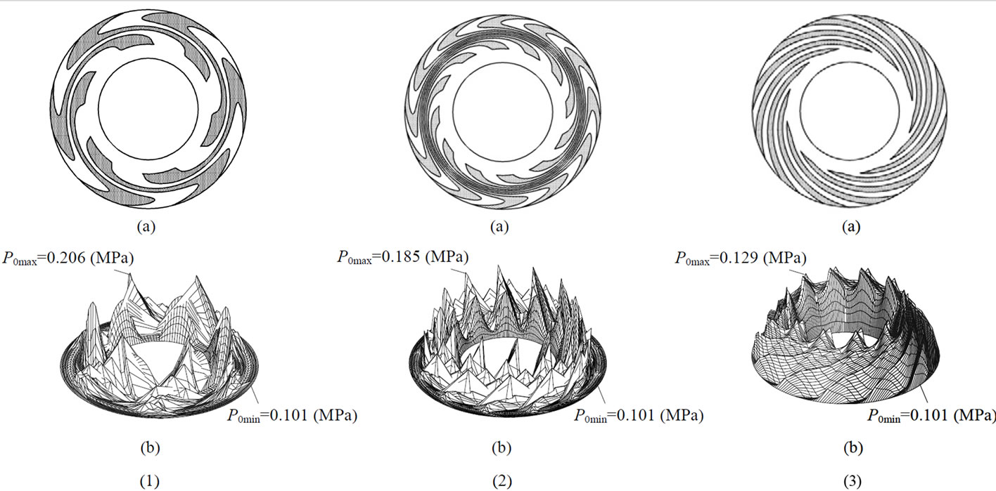
Figure 9. Bearing geometry and static pressure distribution of each optimum design and spiral grooved bearing (initial groove), (1) Robust optimum design considering tolerance (tolerance range, Dhg = ±1.0 mm, Da = ±0.05 ), (2) Optimum design neglecting tolerance and (3) Spiral grooved bearing; (a) Groove geometry and (b) Static pressure distribution.

Table 2. Optimized results
manufacturing costs due to easy manufacturing of bearing grooves.
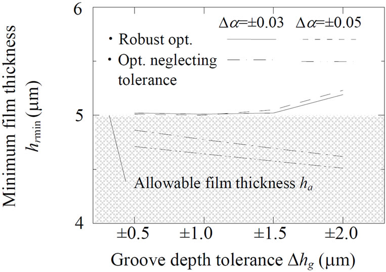
Figure 10 shows a comparison of the results of robust optimum design and optimum design neglecting tolerance. In the figures, (a), (b) and (c) show the minimum oil lubricating film thickness within variability, the variability of bearing stiffness and the expectation of bearing stiffness, respectively.
As can be seen in Figure 10(a), the values of minimum film thickness obtained by the optimum design neglecting tolerance are less than the allowable film thickness. On the other hand, the values of the robust optimum design are exceeded the allowable film thickness for all tolerances. This means that there is a low risk of contact between the bearing and housing when the bearings are manufactured within the setting ranges of tolerance.
In Figure 10(b), the vertical axis shows the ratio of expectation value and standard deviation of bearing stiffness. This means that when the ratio becomes smaller, the expectation becomes larger and standard deviation becomes smaller. The values of ratio obtained by the robust optimum design are less than the ratio by the optimum design neglecting tolerance. In addition, the tendency of ratio becomes flat and the values have not increased for all tolerances of groove depth. As a result, it is confirmed that the robust optimum design is effective of suppressing the variability of bearing stiffness.
As can be seen in Figure 10(c), the expectation of bearing stiffness by the robust optimum design is equivalent to the value neglecting tolerance when the tolerance of groove depth is set within Δhg = ±1.5 μm. On the other hand, the value is decreased from Δhg = ±1.5 μm to Δhg = ±2.0 μm. Because the relationship between the oil film thickness and the bearing stiffness is trade-off, the expectation of bearing stiffness is decreased with increasing the minimum oil film thickness in the tolerance range as
 (a)
(a)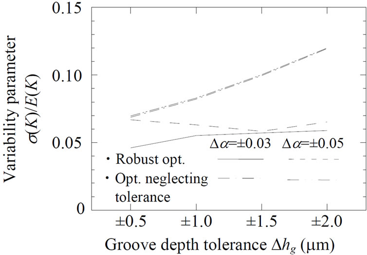 (b)
(b)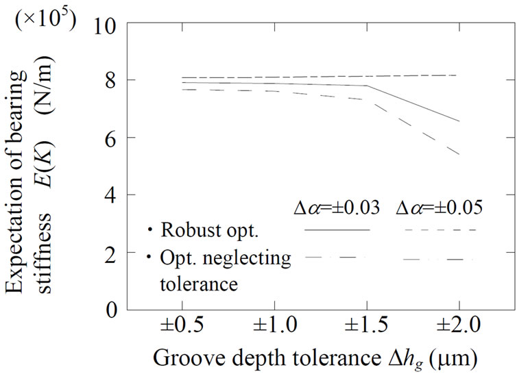 (c)
(c)
Figure 10. Comparison of results of robust optimum design considering tolerance and optimum design neglecting tolerance: (a) Minimum oil lubricating film thickness; (b) Variability of bearing stiffness; and (c) Expectation of bearing stiffness.
shown in Figure 10(a). The reason why such result obtained is because of suppressing the variability of bearing stiffness by Equation (12). Consequently, the tolerance of groove depth of Δhg = ±1.5 μm is recommended to suppress the variability with high bearing stiffness.
6. Conclusions
This paper described the methodology and sample of robust optimum design considering dimensional tolerance based on the statistical method combined with the geometrical optimization for thrust hydrodynamic bearings of a 2.5″ HDD spindle motor. The conclusions are briefly summarized as follows.
1) The optimized groove geometries obtained by the robust optimum design and by the conventional optimum design neglecting tolerance are the modified spiral groove with bends in the vicinity of the outer circumference of the bearing. The bearing stiffness of the modified spiral groove bearing becomes more than four times compared with the stiffness of spiral groove bearing.
2) It is possible to determine the diameter of industrial tool under product design by providing the constraint condition for groove width.
3) The expectation of bearing stiffness by the robust optimum design is equivalent to the value neglecting tolerance, and the standard deviation can be suppressed compared with the standard deviation neglecting tolerance when the bearings are manufactured within the tolerance of groove depth of Δhg = ±1.5 μm.
REFERENCES
- K. Ono and J. Zhu, “A Comparison Study on Characteristics of Five Types of Hydrodynamic Oil Bearing for Application to Hard Disk Drive Spindles,” Transactions of the Japan Society of Mechanical Engineers, Series (C), Vol. 64, No. 622, 1998, pp. 339-345.
- J. Zhu and K. Ono, “A Comparison Study on the Performance of Four Types of Oil Lubricated Hydrodynamic Thrust Bearings for Hard Disk Spindles,” Transactions of the ASME, Journal of Tribology, Vol. 121, No. 1, 1999, pp. 114-121. doi:10.1115/1.2833790
- K. Matsuoka, S. Obata, H. Kita and F. Toujou, “Development of FDB Spindle Motors for HDD Use,” IEEE Transactions on Magnetics, Vol. 37, No. 2, 2001, pp. 783-788. doi:10.1109/20.917616
- G. H. Jang, S. H. Lee, H. W. Kim and C. S. Kim, “Dynamic Analysis of a HDD Spindle With FDBs Due to the Bearing Width and Asymmetric Grooves of Journal Bearing,” Microsystem Technologies, Vol. 11, No. 7, 2005, pp. 499-505. doi:10.1007/s00542-005-0606-5
- T. Hirayama, S. Sakai, N. Yamaguchi, N. Hishida and H. Yabe, “A Proposal of Optimum Groove Design Concepts of Spiral-Grooved Journal Bearings Applied to Spindles of Precision Equipments (1st Report, A Guide for Reduction of Amplitude of Repeatable Run-Out in Incompressible Fluid Film Bearing),” Transactions of the Japan Society of Mechanical Engineers, Series (C), Vol. 72, No. 713, 2006, pp. 241-246. doi:10.1299/kikaic.72.241
- H. Yabe, T. Hirayama, S. Sakai, N. Yamaguchi and N. Hishida, “A Proposal of Optimum Groove Design Concepts of Spiral-Grooved Journal Bearings Applied to Spindles of Precision Equipments (2nd Report, A Guide for Reduction of Amplitude of Indicial Response),” Transactions of the Japan Society of Mechanical Engineers, Series (C), Vol. 72, No. 719, 2006, pp. 312-317.
- S. Tohma, T. Isogai, T. Hirayama, T. Matsuoka, K. Yokozuka and S. Mori, “Frequency Analysis of Hard Disk Drive Spindle System Supported by Hydrodynamic Bearings,” Journal of Advanced Mechanical Design, Systems, and Manufacturing, Vol. 1, No. 5, 2007, pp. 717-725. doi:10.1299/jamdsm.1.717
- H. Hashimoto and M. Ochiai, “Optimization of Groove Geometry for Thrust Air Bearing to Maximize Bearing Stiffness,” Transactions of the ASME, Journal of Tribology, Vol. 130, No. 3, 2008, pp. 1-11. doi:10.1115/1.2913546
- M. D. Ibrahim, T. Namba, M. Ochiai and H. Hashimoto, “Optimum Design of Thrust Air Bearing for Hard Disk Drive Spindle Motor,” Journal of Advanced Mechanical Design, Systems, and Manufacturing, Vol. 4, No. 1, 2009, pp. 70-81. doi:10.1299/jamdsm.4.70
- K. Y. Koak, G. H. Jang and H. W. Kim, “Whirling Tilting and Axial Motions of a HDD Spindle System Due to the Manufacturing Errors of FDBs,” Microsystem Technologies, Vol. 15, No. 10-11, 2009, pp. 1701-1709. doi:10.1007/s00542-009-0872-8
- M. Fillon, W. Dmochowski and A. Dadouche, “Numerical Study of the Sensitivity Tilting-Pad Journal Bearing Performance Characteristics to Manufacturing Tolerances: Steady-State Analysis,” STLE Tribology Transactions, Vol. 50, No. 3, 2007, pp. 387-400. doi:10.1080/10402000701429246
- W. Dmochowski and M. Fillon, “Numerical Study of the Sensitivity Tilting-Pad Journal Bearing Performance Characteristics to Manufacturing Tolerances: Dynamic Analysis,” STLE Tribology Transactions, Vol. 51, No. 5, 2008, pp. 573-580. doi:10.1080/10402000801947709
- W. Xu, P. J. Ogrodnik, M. J. Goodwin and G. A. Bancroft, “The Stability Analysis of Hydrodynamic Journal Bearings Allowing for Manufacturing Tolerances. Part1: Effect Analysis of Manufacturing Tolerances by Taguchi Method,” Proceedings of Measuring Technology and Mechatronics Automation 2009, Vol. 2, Zhangjiajie, 11- 12 April 2009, pp. 164-167.
- P. J. Ogrodnik, M. J. Goodwin, G. A. Bancroft and W. Xu, “The Stability Analysis of Hydrodynamic Journal Bearings Allowing for Manufacturing Tolerances. Part2: Stability Analysis Model with Consideration of Tolerances,” Proceedings of Measuring Technology and Mechatronics Automation 2009, Vol. 2, Zhangjiajie, Hunan, 11-12 April 2009, pp. 168-171.
- G. J. Park, T. H. Lee, H. L. Kwon and K. H. Hwang, “Robust Design: An Overview,” American Institute of Aeronautics and Astronautics, Vol. 44, No. 1, 2006, pp. 181-191.
- H. Hashimoto and M. Ochiai, “Theoretical Analysis and Optimum Design of High Speed Gas Film Thrust Bearings (Static and Dynamic Characteristic Analysis with Experimental Verifications),” Journal of Advanced Mechanical Design, Systems, and Manufacturing, Vol. 1, No. 1, 2007, pp. 102-112. doi:10.1299/jamdsm.1.102
- N. Kawabata, “Study on Generalization of Calculations of Lubricant Flow Using Boundary Fitted Coordinate System (Part 1, Basic Equations of DF Method and Case of Incompressible Fluids),” Transactions of the Japan Society of Mechanical Engineers, Series (C), Vol. 53, No. 494, 1987, pp. 2155-2160
Appendix I
The cubic spline function is a cubic polynomial equation in each section of 
 . The condition required for the cubic spline function is a continuity of the second order derivative of the function at each nodal point.
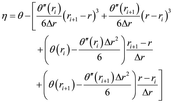
The cubic spline interpolation function is expressed as the following equation.
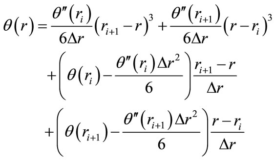 (I-1)
(I-1)
Considering that 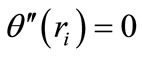 for
for  and
and ,
, 
 are given as follows:
 (I-2)
(I-2)
where
 (I-3)
(I-3)
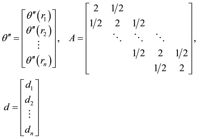
where d in Equation (I-3) is expressed as the following.
 (I-4)
(I-4)
 (I-5)
(I-5)
 (I-6)
(I-6)
An arbitrary groove geometry can be represented by finding the spline function in all sections of the target groove geometry using Equations (I-1) and (I-2).
Appendix II
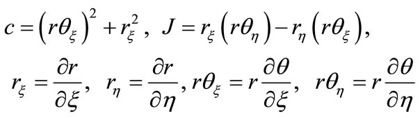
When optimizing the groove geometry, it is necessary to perform a sequential analysis of characteristics of a bearing with a groove geometry modified in succession by the finite difference method, but because of the r-θ polar coordinate system, direct processing is rather different to realize. Therefore, an analysis of the bearing stiffness is performed first by using a boundary-fitted coordinate system as shown in Figure 11 [16,17] and transforming a complex groove geometry into a simple fanlike geometry. A boundary transformation function used for the transformation is given as
 (II-1)
 (II-2)
The following Reynolds equivalent equation can be obtained from the equilibrium between the mass flow rates of oil inflowing into and outflowing from the control volume due to the shaft rotation and the squeezing motion:
 (II-3)
where ,
,  indicate the mass flow rates, across the boundary of
  = const. and across the boundary of
  = const. as shown in Figure 12. On the other hand,
  indicates the mass flow rate due to squeezing motion inside the control volume.
 ,
,  and
and  are expressed, respectively, as follows:
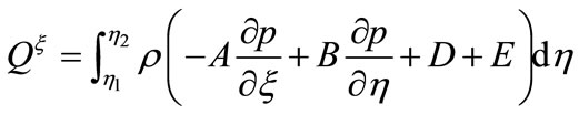 (II-4a)
 (II-4b)
 (II-4c)
In that case,

 (II-4c)
Then, in Equation (II-3), subscripts l and 2 and I-IV
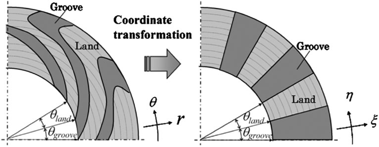
(a) Original bearing geometry (b) Transformed bearing geometry
Figure 11. Bearing geometry transformation based on the boundary-fitted coordinate system.
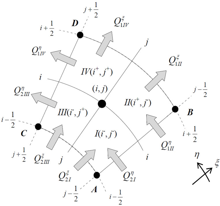
Figure 12. Definition of control volume.
indicate the domains in the control volume.
Assuming that variations of the bearing clearance are microscopic, the minimum oil lubricating film thickness h and pressure p can be expressed by the following equation:
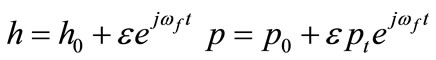 (II-6)
In that case, ε indicates the amplitude of small variations of the oil lubricating film thickness and p0 and pt express a static component and a dynamic component, respectively.
The substitution of Equation (II-6) into Equation (II-3) and the negligence of terms of small magnitude of ε of above second order allow the introduction of two equations for terms ε of orders 0 and l as follows:
 (II-7a)
 (II-7b)
In that case, subscript 0 indicates a static component of the mass flow rate determined from Equation (II-4) and subscript t similarly indicates a dynamic component.
Solving Equations (II-7a) and (II-7b) in turns by the Newton-Raphson iteration method, the static and dynamic components, p0 and pt, are obtained.