Journal of Environmental Protection
Vol. 3 No. 9A (2012) , Article ID: 22987 , 6 pages DOI:10.4236/jep.2012.329144
Driving Cycle for Motorcycle Using Micro-Simulation Model*
![]()
1CSIR-Central Road Research Institute, New Delhi , India; 2Transport Research Institute, Edinburgh Scotland, UK.
Email: ravindra261274@yahoo.co.in
Received June 7th, 2012; revised July 31st, 2012; accepted August 2nd, 2012
Keywords: Micro-simulation; driving cycle; vehicular emission; motorcycle
ABSTRACT
Driving cycle of vehicle has been used in emission estimation and fuel consumption study. Existing method of data collection using car chasing technique is expensive. The technique using micro simulation approach is cheaper and fast to derive the driving cycle. In this paper a traffic simulation model Driving Cycle Micro-Simulation Model for Motorcycle has been developed. The issue of lateral and longitudinal movement aspect in motorcycle driving has been examined in the model. Parameters to cover such movement have been built in the model and applied on a stretch in Edinburgh city of Scotland. Results from model have been both calibrated and validated. The results show that Driving Cycle Micro-Simulation Model for Motorcycle gives better representation of driving cycle and it can be used to understand the effect of driving modes on emission for better understanding of vehicular emission control.
1. Introduction
This Traditional chase car method, and on board method for data collection of driving cycle are expensive in nature [1]. Traffic micro-simulation models can simulate/ represent individual driver behavior and the real world driving cycles in laboratory for vehicles and roads in cost effective manner using secondary data [2]. Modelling individual driving cycle for motorcycle is done by simulating the speed of vehicles second-by-second basis. In this paper, Driving Cycle Micro-Simulation Model for Motorcycle (DCMSMM) for a section of urban network in Edinburgh has been developed. Its calibration and validation has been done using different sets of realworld data of driving cycle of Edinburgh Motorcycle Driving Cycles (EMDC) and results of DCMSMM have been compared with published parameters of EMDC [1] and corresponding emission factor (EF) are evaluated.
2. Model Building
2.1. Selecting a Parameters for Model Development
In most of the microscopic traffic simulation model, longitudinal dynamics of single vehicles parameters influence the model. But, the movement of motorcycles is a two-dimensional movement i.e. longitudinal and lateral movement. The longitudinal movement contributes to forward movement and lateral movements are used to take up appropriate positions. Motorcycles can get more longitudinal gap to accelerate their speed by lateral movements [3]. In another case study of Edinburgh driving cycle for motorcycle of Gorgie Road of 1.01 km length having signal free section were developed by Kumar [4]. They investigated simulation of motorcycle driving behaviour and found the average speed 17.37 km∙h−1, proportion of idling time 35%, and time spent in proportion of acceleration was found to be 35.8%.
However the results were neither calibrated nor validated. But this case study was good application of microsimulation approach to develop driving cycle for motorcycles.
In this paper VISSIM 5.10 has been used for simulation and additional required parameters have been created to derive the speed-time sequence representing driving cycle for motorcycle. The motorcycle traffic flow is influenced by driver characteristics, vehicle interactions and the external environment, all of these the proposed model DCMSMM are taken into account. The vehicle interactions such as longitudinal and lateral movements, external environment as creation of motorcycle lanes near the stop line for its stopping in front are considered in model building.
2.2. Inputs for DCMSMM
There are four required input i.e. traffic signal, road-network, driver behaviour and vehicular characteristic and behaviour characteristics to create the microscopic motorcycle driving cycle model. The detailed driver behaviour look ahead distance, the maximum distance allowed for looking ahead, the minimum value minimum look ahead distance, the observed vehicles and look back and other parameters gap, headway etc. are exclusively needed to model lateral vehicle behaviour (Table 1). Routes and nodes are created on existing routes. Database of traffic video, signal time and traffic flow for 21 intersections for section of the AQMA area of Edinburgh is developed and used as input to simulate driving cycle. Parking lots are created to start the point at Morningside-Holy Corner road to end point at Broughton Street for simulation run of motorcycle. Range of relevant traffic parameters such as driving behaviour parameters, simulation parameters such as random seeds, time scale are extracted from database and used for further analysis and model calibrations, till simulation results are stabilised.
The following factors are considered as assumption in modelling while comparing with real world driving cycle 1) Geographical characteristics of modelled corridor 2) Length of the corridor 3) Type of engine size 4) Driving behaviour 5) Signal control 6) Time of survey 7)Traffic assignment. Table 1 shows requisite changes made in simulation parameters of driving behaviour for motorcycles to generate motorcycle driving cycles. Finally simulation models are run with simulation resolution of 1-Second and with different random seeds.
2.3. Characteristics of Study Area
Series of micro simulation runs were made along Edinburgh AQMA corridor (Figure 1). The test track covered nineteen traffic signals (one 5-arm, seven 4-arm and ten T-junctions). The speed limit is 48 km∙h−1 along the corridor and total percentage of motorcycle traffic varies from 1% - 3% of the total fleet. The part of test track is used for developing the driving cycle for motorcycles-EMDC [1]. GPS based data acquisition system was installed in
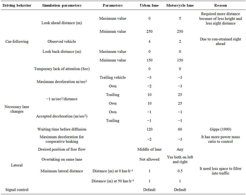
Table 1. Change in default simulation driving behavior parameter for urban and motorcycle lane.
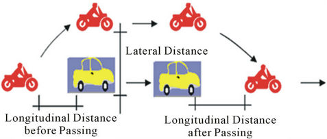
Figure 1. Passing maneuvers of motorcycles.
motorcycle for field data collection for calibration and results validation. Signal cycle length significantly affect the cycle time of driving cycles, their phase wise data were collected to build the model.
2.4. Calibration and Validation of DCMSMM
Calibration and validation of driving cycle simulation model for motorcycle is done by GEH technique [5-7] which is frequently used by Directorate of Traffic Operations (DTO) in UK [8]. GEH value of 5 indicates a good level of threshold reliability and The GEH statistic is standard measure of the “goodness of fit” between observed and modelled flow. The GEH is calculated as follows in “Equation (1)”
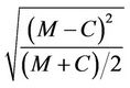 (1)
(1)
where M and C are the modelled and observed speed (% frequency) respectively.
Smaller GEH values indicate a better “fit” between observed and modelled speed [8]. Table 2 shows the GEH values for the reliability indicator. Two data sets are compared; real world speed and the modelled speeds from simulation model. Observed speeds from both real world and DCMSMM are categorized into seven categories for speed ranges between 0 - 60 km∙h−1. The GEH statistics are applied on the results from simulation. Four values of random seeds were used for GEH statistical goodness of fit. Different random seeds are considered in simulation run. The corresponding speed frequency by changing the value of random seeds (90, 30, 50, and 10) is estimated. The speeds are found in the range of 0 - 10 km∙h−1 and 10 - 30 km∙h−1 which is lower than the realworld driving speed. The real world driving cycle’s speeds are found to be distributed in the range of 0 - 20 km∙h−1 and 30 - 69 km∙h−1. Little deviation between real world and micro-simulation approach is observed. Models with the same number of random seeds and input files have the same result, but the different random seeds with same input files will have different result and vice versa, because random seeds affect the realization of the stochastic quantities in simulation such as inlet flows and vehicle capabilities.
2.5. The Model Outputs
The output files from micro-simulator run are recorded for each vehicle’s actions. DCMSMM provide the instantaneous speed data at intervals of 1 second or 0.1 second for each individual vehicle. In data analysis, simulation resolution is assigned one second to create the smooth driving pattern. The final value of random seed is selected when simulated results get stabilize. Figure 2 shows simulated speed of DCMSMM, which is able to reproduce the real-world speed time sequence of the motorcycle driving cycle. The model outputs are integrated with National Atmospheric Emission Inventory (NAEI) database to estimate emission. The instantaneous speed from micro-simulation approach is useful to estimate the emissions in the absence of on-board measurement or laboratory measurement.
3. Results and Discussions
3.1. Characteristic of DCMSMM
Table 3 present comparisons of characteristics of the DCMSMM with Edinburgh Real World Motorcycle Cycle Driving Cycle-EMDC [1]. A large proportion of the DCMSMM cycle time is found in cruising while time spent in idling time is relatively small. The average cycle speed over the whole driving cycle (V1) is 14.4 km∙h−1, while the average running speed (V2) is 18.22 km∙h−1. Average acceleration is 0.65 ms−2, while average deceleration is 0.556 ms−2. The mean length of driving period is 1010 second (around 16 minutes).Total driving length is 4.1 km. It should be noted that micro-simulation based methodology is highly sensitive and needs many parameters for calibration and validation. The more parameters are available for the calibration of driving cycle, the higher the accuracy would be. However, the comparison should be taken with great care, since there are a number of assumptions, affect the accuracy of the results. Table 3 present the value of assessment parameters of EMDC and simulated driving cycles.
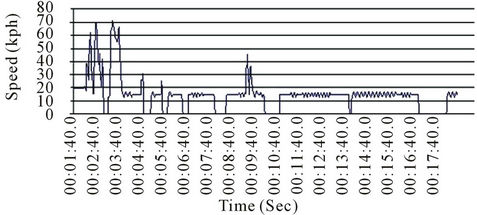
Figure 2. Simulated driving cycle of motorcycle for Edinburgh AQMA.
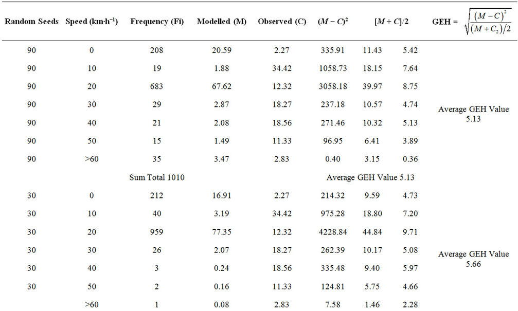
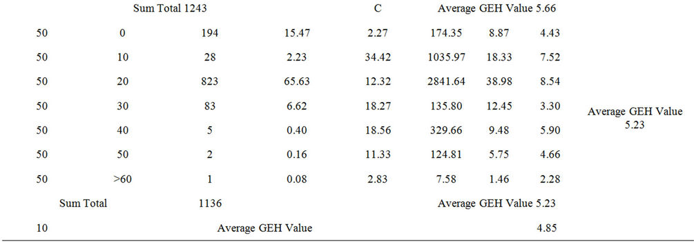
Table 2. GEH value for calibration of micro-simulation model.
3.2. Comparison of Driving Cycle Parameter for Simulated and Real World
The average speed (V1) and average running speed (V2) in the simulated driving cycle are found to be nearly half that of the real-world driving cycle. The total cycle duration is from 1010 seconds in the simulated driving cycle where as it is 770 second in real-world EMDC. Time is spent in idling for DCMSMM is found higher in city centre. Therefore, cycle time of the real world and the simulated cycles is different. Time spent in idling is found 18% of the total cycle time, which deviates noticeably from the real-world value (1.5%). The percentage of time spent in acceleration is found to be 24% as compared to 44.5% in the EMDC. In contrast, percentage of time spent in deceleration for DCMSMM simulated is 28% as compared to 46.87% in the EMDC. However, the cruising proportion of the EMDC is found to be 7.24%, extremely low compared to 29.45% for the simulated cycle. In simulated system, there is no representation of the SCOOT system and real world assignment of traffic volume on all the arms, therefore the results deviate strongly. The number of changes in acceleration and deceleration in one driving period in simulation is found to be much lesser than the real-world cycle, which indicates that drivers are sensitive to the traffic, signals, and other
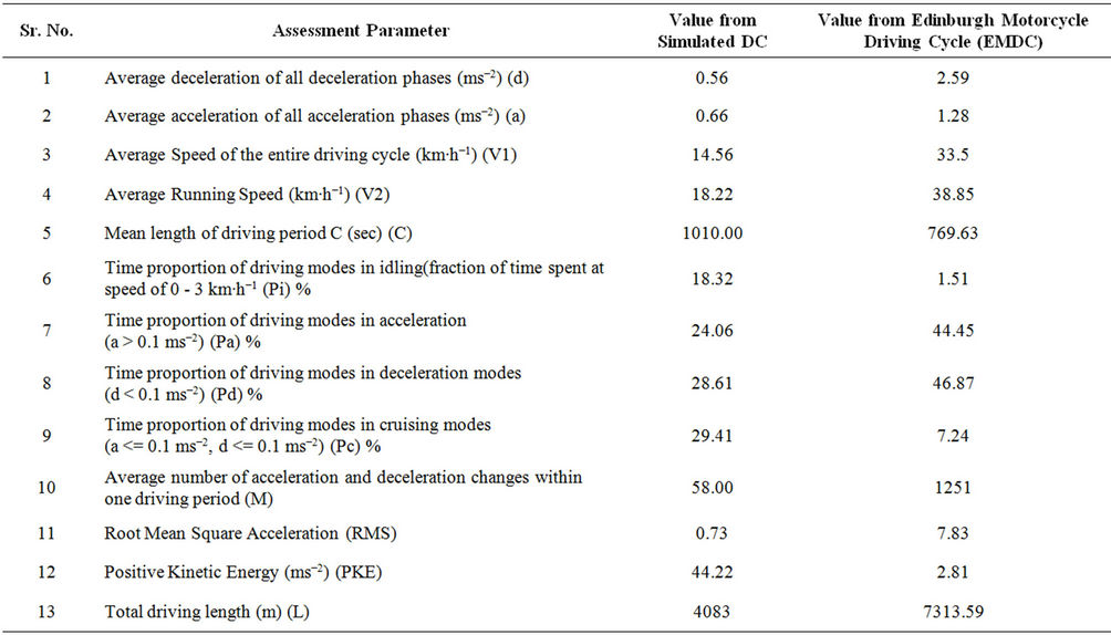
Table 3. Characteristics of driving cycle.
factors in the real world [1,9,10].
3.3. Effect of Driving Modes on Emission
The quantities and composition of emission product from vehicles depend on the mode of driving (See Table 4). Normally, when the test vehicle starts from the cold, the fuel enrichment increases in choke that provides an easily-combustible mixture near the spark plug. It happens due to slow vaporization of fuel. However, nitric oxide concentration during these modes is low because of low temperature and scarcity of oxygen in the engine. The four modes of driving have been classified 1) time spent in acceleration 2) time spent in deceleration 3) time spent in cruise 4) time spent in idling based on the parameters defined in Tong et al. [11]. The simulated driving cycle has 18.46% of time spent in idling. Time spent in deceleration and acceleration is almost equal. There is increase in emission factors during cruising mode except in the case NOX. HC emission factor is in the range of 1.67 gm/km and CO2 is found in the range of 148 to 152 gm/km. NOX emission factors are lowest with 0.302 to 0.2 gm∙km−1. CO emission factor is found between 26.49 to 26.0 gm∙km−1. The average value of CO, HC and NOX emissions (gm∙km−1) for the 1000 cc engine are estimated 26.7, 1.72 and 0.283 gm∙km−1 respectively, whereas CO, HC and NOX emissions (gm∙km−1) for 600 cc are 10.581, 1.90 and 0.283 gm km-1 respectively. All three pollutants showed higher value than existing regulatory standard. EF of HC is found to be higher than simulated EF whereas EF of NOX for 600 cc engine shows extremely higher even more than Euro 1 standard. Such event can be attributed to induction of Extra Urban Driving cycle in Euro 2 engine size unless NOX catalyst is not activated.
4. Conclusion
Driving Cycle Micro-Simulation Model for Motorcycle (DCMSMM) is important in understanding emission in different driving modes. Real time data and simulated driving cycle data are compared. Calibration and validation of DCMSM shows its capability to represent realistic driving cycle. However there are several assumptions made in modeling; such type of exercise is very effective in better understanding the driving behavior of motorcycle. Understanding longitudinal and lateral movement of
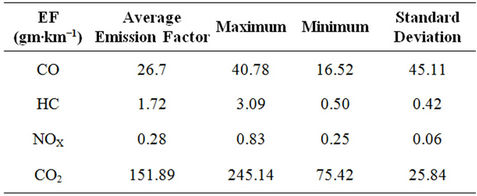
Table 4. Observed emission factors from simulated driving cycle using NAEI coefficient.
motorcycle and model in computer simulated platform is challenging task because of involvement of many input parameters. The comparison with real world data shows nearby results but assumption made bring attention to modeller for better input parameters and more number of simulation runs.
5. Acknowledgements
Dr. Ravindra Kumar thanks Director CRRI to allow publishing this paper. Other team members who have helped us directly and indirectly are duly acknowledged.
REFERENCES
- W. Saleh, et al., “Real World Driving Cycle for Motorcycles in Edinburgh,” Transportation Research Part D, Vol. 14, No. 5, 2009, pp. 326-333. doi:10.1016/j.trd.2009.03.003
- P. Hidas, “Modelling Vehicle Interactions in Microscopic Simulation of Merging and Weaving,” Transportation Research Part C: Emerging Technologies, Vol. 13, No. 1, 2005, pp. 37-62. doi:10.1016/j.trc.2004.12.003
- T.-C. Lee, et al., “New Approach to Modeling Mixed Traffic Containing Motorcycles in Urban Areas,” Journal of the Transportation Research Board, Vol. 2140, 2009, pp. 195-205. doi:10.3141/2140-22
- R. Kumar, et al., “Development of Driving Cycle for Motorcycle for Edinburgh World Association for Sustainable Development,” 5th International Conference Managing Knowledge, Technology and Development in the Era of Information Revolution Griffith University, Gold Coast, 2007, pp. 357-364.
- C. Barcelo, et al., “Methodological Notes on the Calibration and Validation of Microscopic Traffic Simulation Model,” Proceeding of 83rd Annual Meeting of Transportation Research Board Annual Conference, Washington DC, 2004.
- L. Chu, et al., “Using Microscopic Simulation to Evaluate Potential Intelligent Transportation System Strategies under Non recurrent Congestion,” Journal of the Transportation Research Board, Vol. 1886, 2004, pp. 76-84. doi:10.3141/1886-10
- T. Oketch, and M. Carrick, “Calibration and Validation of a Micro-Simulation Model in Network Analysis,” Proceedings of the 84th TRB Annual Meeting, Washington DC, 2005.
- DTO (Directorate of Traffic Operations), “Modelling Guidelines Version 2.0 Traffic Schemes in London Urban Networks,” Transport for London Surface Transport, 2006.
- R. Kumar, et al., “Comparison and Evaluation of Emissions for Different Driving Cycles of Motorcycles: A Note,” Transportation Research Part D: Transport and Environment, Vol. 16, No. 1, 2011, pp. 61-64. doi:10.1016/j.trd.2010.08.006
- W. Saleh, et al., ““Real-World Driving Cycle for Motorcycles: A Comparative Study between Delhi and Edinburgh” World Journal of Science, Technology & Sustainable Development, Vol. 7, No. 3, 2010, pp. 263-274.
- H. Y. Tong, et al., “On-Road Motor Vehicle Emissions and Fuel Consumption in Urban Driving Conditions,” Journal of Air Waste Management Association, Vol. 50, No. 4, 2000, pp. 543-554. doi:10.1080/10473289.2000.10464041
NOTES
*Micro-simulation based driving cycle derivation for motorcycle.