Journal of Applied Mathematics and Physics
Vol.03 No.11(2015), Article ID:61587,19 pages
10.4236/jamp.2015.311179
Comparison of Finite Difference Schemes for the Wave Equation Based on Dispersion
Yahya Ali Abdulkadir
Department of Physics, University of Gondar, Gondar, Ethiopia

Copyright © 2015 by author and Scientific Research Publishing Inc.
This work is licensed under the Creative Commons Attribution International License (CC BY).


Received 23 September 2015; accepted 27 November 2015; published 30 November 2015

ABSTRACT
Finite difference techniques are widely used for the numerical simulation of time-dependent partial differential equations. In order to get better accuracy at low computational cost, researchers have attempted to develop higher order methods by improving other lower order methods. However, these types of methods usually suffer from a high degree of numerical dispersion. In this paper, we review three higher order finite difference methods, higher order compact (HOC), compact Padé based (CPD) and non-compact Padé based (NCPD) schemes for the acoustic wave equation. We present the stability analysis of the three schemes and derive dispersion characteristics for these schemes. The effects of Courant Friedrichs Lewy (CFL) number, propagation angle and number of cells per wavelength on dispersion are studied.
Keywords:
Wave Equation, Finite Difference Methods, Dispersion

1. Introduction
Real life situations in many disciplines including engineering, physics, economics, biosciences, etc, can be described through mathematical models. Differential equations play an important role in modelling interactions in physics, engineering, and biological processes, from ground motion (earthquake) to interactions between neurons. Differential equations can either be categorized as ordinary differential equations (ODEs), which are for example, used to model dynamical systems and their applications to science and engineering or partial differential equations (PDEs), which most importantly used to describe a wide variety of phenomena in physics; such as sound, heat, fluid dynamics, elasticity and in most field of engineering in general. However, most differential equations, such used to solve real-life problems, have no analytical solutions or are unrealistic to solve analytically. Therefore, solutions for these problems are attempted by means of numerical approximations. To this end various numerical methods are developed to provide better approximate solutions to these equations.
Numerical techniques are a powerful tool for handling large systems of equations involving complex geometries that are otherwise impossible to handle analytically [1] . There are several types of numerical methods, each with their own pros and cons. Finite difference method (FDM) is the most popular numerical technique which is used to approximate solutions to differential equations using finite difference equations [2] . These techniques are widely used for the numerical solutions of time-dependent partial differential equations. However, when we approximate derivatives using finite difference methods truncation of terms produces inaccuracies. Due to these truncations an inherent problem arises, undesirable ripples are produced due in the process of discretization. Sometimes, due to truncation of higher order terms, frequency dependent numerical errors called dispersion is produced. A large amount of work has been developed for higher order accurate scheme with low dispersion; for instance, Krum [3] developed time-domain schemes based on multiresolution analysis, Lee [4] introduced a low-dispersive schemes based on Pseudo-spectral approach.
The aim of this research is to explore a higher order compact finite difference scheme with comparably low dispersive characteristics. Therefore, in this paper, firstly, we discussed a conventional higher order finite difference schemes. Then we discussed another higher order finite difference scheme developed by Das [5] and Liao [6] . We also discussed the dispersion properties of these methods by comparing with a conventional higher order finite difference scheme. The paper explores comparably low dispersive scheme with among the finite difference schemes.
2. Higher Order Finite Difference Discretization for the Wave Equation
The two dimensional version of the wave equation with velocity v and acoustic pressure u in homogeneous media can be written as
 (1)
(1)
where , along with the initial conditions
 (2)
(2)
 (3)
(3)
and the boundary condition
 (4)
(4)
3. Finite Difference Operators
To discretize the above PDE we consider a uniform grid  equally spaced in all spacial direction with a grid spacing
 ; N is number of grid points, τ and
  denotes the time-step and the numerical approximation of
 , respectively.
The central finite difference operators for second derivatives are written as [7]
 (5)
(5)
 (6)
(6)
 (7)
(7)
A higher order finite difference approximation for the second derivative is given by Liu [8] .
 (8)
(8)
 (9)
(9)
where  and
and  are central difference coefficients. Some values of these coefficients are presented in Table 1, and the formula to find all coefficients can be found in Liu [8] .
Though this approximation is accurate up to order 2M, its not efficient because when M becomes large, the stencil that need to be computed becomes large.
The standard second-order finite difference approximation for the acoustic wave equation in (1) using the above operators is
 (10)
(10)
 (11)
(11)
where  is the Courant Friedrichs Lewy(CFL) number with
 .
.
4. Implicit Finite Difference Method
A fourth order accurate implicit finite difference scheme for one dimensional wave equation is presented by Smith [9] . We extend the idea for two-dimensional case as discussed below.
Consider two dimensional wave equation, using Taylor’s series expansion of  and
and  about the point
  we have
 (12)
(12)
If u is a solution of (1), then we have the following
 (13)
(13)
and
 (14)
(14)
Substituting equations (13) and (14) in to equation (12) and using the notations


and

Table 1. Coefficients of central difference formula.

we obtain
 (15)
(15)
Following Strikwerda [10] and using Taylor’s series expansion we obtain
 (16)
(16)
and
 (17)
(17)
We also have
 (18)
(18)
an
 (19)
(19)
Substituting (16)-(19) into (15) gives a scheme which is fourth order accurate
 (20)
(20)
where  as denoted above.
Applying the operator

to both sides of (20), we obtain
 (21)
(21)
Equation (21) can be written as an ADI-scheme and can be referred to as HOC-ADI, which can be presented more precisely as,
 (22)
(22)
 (23)
(23)
We have introduced the higher order finite difference alternating direction implicit scheme for two-dimension- al wave equation. In the next section we will derive another higher order scheme based on Padé approximations.
5. Higher Order Finite Difference Scheme Based on Padé Approximation from Taylor’s Series Expansion We Have
 (24)
(24)
 (25)
(25)
 (26)
(26)
Therefore,
 (27)
(27)
Similarly the discretization in the t, y and z directions are
 (28)
(28)
 (29)
(29)
substituting (27)-(29) into (1) we have
 (30)
(30)
The scheme presented in (30) is a 4th-order accurate both in time and space for the 2-dimensional acoustic wave equation based on Padé approximation.
6. Higher Order Compact Finite-Difference Method for the Wave Equation
A compact finite difference scheme comprises of adjacent point stencils of which differences are taken at the middle node, therefore typically 3, 9 and 27 nodes are used for compact finite difference descretization in one, two and three dimensions, respectively. Whereas a non-compact stencil comprises of any number of nodes which are near the vicinity of the middle node. Usually, when the order of accuracy of a non compact scheme is greater than two, then the scheme is said to be higher order. Figure 1 represents a compact and non-compact stencil in two-dimensions.
6.1. Higher Order Compact Alternating Direction Scheme for the Wave Equation
The standard alternating direction implicit scheme which is fourth order both in time and space is given in equa- tion (22)-(23). Recently, Das [5] developed a low dispersive finite difference method for two-dimensional a

Figure 1. Compact (left) and Non-compact (right) stencils.
coustic wave equation using Padé approximation, we will discuss this method in detail.
Multiplying both sides of (30) by the operator

we get
 (31)
(31)
which upon simplification leads to
 (32)
(32)
Further simplification give
 (33)
(33)
Neglecting the term  which is equivalent to an error of
  we obtain the compact
scheme, which is fourth order in time and space,
 (34)
(34)
This scheme needs to be solved in two directions simultaneously, however it is easier to solve it in one direction at a time, therefore we can write it as
 (35)
(35)
 (36)
(36)
The above scheme is based on Pad’e approximation and which can be referred to as CPD-ADI scheme.
Substituting (16) into (36) we obtain
 (37)
(37)
Equation (37) is a tridiagonal system and therefore it can be solved easily by using any tri-diagonal solver.
In the next section we will derive a numerical scheme which is a combination of the compact and non-com- pact operators that we introduced in chapter two.
6.2. Hybrid Scheme
The higher order compact scheme (35)-(36) derived using Padé approximation is efficient and accurate up to order 4. However, the scheme suffers from a moderate numerical dispersion [5] . Therefore, we modify the scheme by substituting one of the spacial grids (in x-direction) in Equation (30) by non-compact one in Equation (8) to obtain a hybrid scheme.
Therefore, for the two-dimensional wave equation we have
 (38)
(38)
Following the same procedure as we did for (32)-(34) we obtain
 (39)
(39)
Therefore, for implementation, this can further be written as an ADI scheme
 (40)
(40)
 (41)
(41)
Equations (40)-(41) is an ADI scheme obtained by mixing compact and non-compact difference operators and therefore it can be referred to as non-compact padé based scheme (NCPD-ADI).
For the implementation, we will apply Equation (40)-(41) for the interior nodes, whereas at the nodes near the horizontal boundary we will use (35)-(36). Therefore, the combination of the two schemes can be called compact Padé based interlinked alternating direction implicit scheme (IPD-ADI).
At this stage, we would like to mention that a typical numerical method may produce spurious solution, a phenomena which is greatly attributed to dispersion. Thus, in the next section we will study this phenomena in detail.
7. Dispersion Relation and Stability Analysis
Finite difference schemes are widely used in solving time dependent partial differential equations numerically, however in approximation of derivatives using Taylor’s series, truncation of terms produces inaccuracies in finding solutions for such differential equations. Due to these inaccuracies undesirable ripples are produced in the process of discretization. Eventhough such equations are not frequency dependent, due to truncation of higher order terms frequency dependent numerical errors are produced. This numerical phenomena is called dispersion. Thus, even for non-dispersive partial differential equations their discrete approximations are dispersive. Moreover in descritizing a differential equation, depending on our interest in accuracy, we ignore higher order terms, due to these inaccuracies errors are introduced which results in instability of the finite difference scheme.
Dispersion Relation
We will consider a scalar wave Equation (1) which has solution of the form
 (42)
(42)
Then its discrete form is given by
 (43)
(43)
where  is pressure amplitude, ω denotes angular frequency,
  is grid spacing, τ is time-step and
discrete directional wave numbers are given by ,
,  ,
, 
and .
.
The dispersion relation is given by
 (44)
(44)
where  is the analytical dispersion relation and we will derive the numerical dispersion relation for two-dimensional wave equation for the mentioned schemes.
In numerical analysis the relation between the numerical angular frequency ω and k, v and numerical parameters τ and h is called numerical dispersion relation.
Dispersion error therefore can be considered as the difference between the numerical and analytical frequencies or the ratio of these frequencies. Consequently, it can be measured as the difference between, or the ratio of numerical and analytical velocities. Since the latter method is the most convenient to work with, we will use this method for our dispersion measurement. Thus, mathematically,
 (45)
(45)
where v is numerical velocity and δ is the normalized phase error.
Therefore  imply the numerical scheme that we are evaluating is non-dispersive, where as for values largely deviating from 1 indicates the scheme is dispersive.
Applying finite difference operators to (43) gives as
 (46)
(46)
 (47)
(47)
 (48)
(48)
For two-dimensional HOC-ADI scheme the phase relation is derived as follows. Substituting (43) into (21) we obtain
 (49)
(49)
 (50)
(50)
 (51)
(51)
 (52)
(52)
Similarly the normalized phase relation for CPD and NCPD schemes in two dimensions respectively are given by
 (53)
(53)
and
 (54)
(54)
where


The plots for these normalized dispersion relations are given in the subsequent sections.
8. Stability Analysis
A numerical scheme is said to be stable if the errors produced, due to descritization, at one time-step of the calculation do not propagate as computation continues. For a stable scheme, the errors decay and eventually damp out, whereas for the unstable scheme the errors grow with time.
In this section we will analyse stability for HOC, CPD and NCPD schemes using Von Neumann stability analysis.
Therefore, the CFL condition for the HOC scheme is derived as follows
Equation (43) can be written as
 (55)
(55)
 (56)
(56)
Substituting (56) in to (21) we obtain
 (57)
(57)
We consider , then (57) can be written as
 (58)
(58)
where
 (59)
(59)
and
 (60)
(60)
For stability the root condition for (58) should be satisfied. Therefore,
 (61)
(61)
Similarly for the CPD scheme we find the stability condition as
 (62)
(62)
where
 (63)
(63)
and
 (64)
(64)
And for the NCPD scheme the stability condition is
 (65)
(65)
where
 (66)
(66)
and
 (67)
(67)
Hence from (61), (62) and (65) we can observe that the three schemes (HOC, CPD and NCPD) are conditionally stable. Note that most of the other finite difference schemes for the acoustic wave equation are conditionally stable, see e.g., [11] [12] .
9. Dispersion Analysis and Discussion
In the previous section, we have discussed the dispersion relation for three finite difference schemes which are HOC, CPD and NCPD schemes. In the next two sections, we will provide a comparison of the dispersion relations of these schemes. We present plots of the dispersion relations as a function of propagation angle θ and number of cells per wavelength (kh) for these schemes. Therefore, we discussed the normalized phase error with respect to different parameters and we approached the comparison of the dispersion errors by plotting the norm of the errors and relative phase errors.
Normalized Phase Error
We can observe that the numerical dispersion of the above mentioned methods are dependent on three variables. Therefore the normalized phase errors for these methods are studied based on these three factors.
• CFL numbers (r)
• Propagation angle (θ)
• Number of cells per wavelength (kh)
• Effect of different CFL number
For the analysis given here, we keep the grid size equal in all spatial directions, i.e.,  and
and . Therefore, by varying r from 0.4 to 1.0 we plot the dispersion error for each scheme. We also used the term ‘exact’ in all the plots for implying that there is no dispersion error, and for NCPD scheme we considered
  for all the plots.
Figure 2 shows the normalized phase error, derived in the earlier section, with respect to kh for HOC-ADI scheme. As clearly observed from the plot, the phase error decreases as CFL number increases; moreover for small kh the phase error decreases for all values of r.
In Figure 3 we plot the normalized phase error for CPD-ADI scheme. As we can closely observe that the plots for HOC-ADI and CPD-ADI for the given parameters shows almost same result.
In Figure 4, we present a plot of the normalized phase error for NCPD-ADI scheme. In this case, the plot for the phase error is different from the above two plots. For  the schemes don’t show phase error for HOC and CPD schemes, whereas for NCPD scheme the plot shows significant phase error.
1) Effect of different propagation angles (θ)
In this subsection, we present plots of the three schemes to study the effect of propagation angle on numerical
dispersion. We choose  and four different values of θ varying from
  to π.
to π.
In Figures 5-7, we provide the normalized phase error with different propagation angles of the wave. We plotted the phase error versus kh for different values of θ varying from  to π. As the plots shows that the propagation angle has a significant contribution for the dispersion errors. It is observed that for
  the HOC-ADI schemes have lower dispersion, whereas CPD-ADI and NCPD-ADI scheme shows low dispersion at
 . It is also shown that CPD-ADI and NCPD-ADI schemes have relatively low dispersion errors for larger kh values than HOC-ADI scheme.
2) Effect of different number of cells per wavelength (kh)
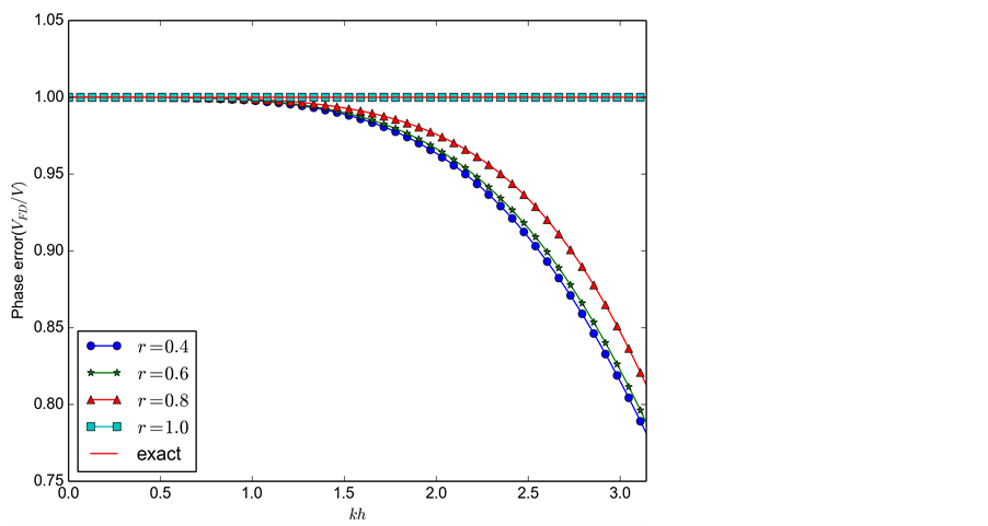
Figure 2. Normalized phase error for different CFL numbers for HOC-ADI scheme, θ = 0˚.
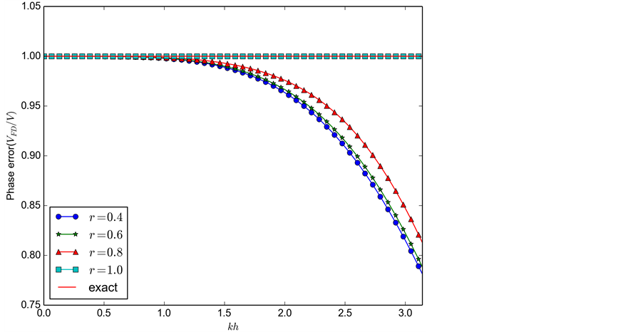
Figure 3. Normalized phase error for different CFL numbers for CPD-ADI scheme, θ = 0˚.
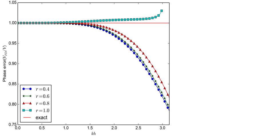
Figure 4. Normalized phase error for different CFL numbers for NCPD-ADI scheme, θ = 0˚.
To examine the effect of number of cells per wavelength, we plot the dispersion errors versus θ for different values of number of cells per wavelength for the three schemes.
In Figures 8-10 we presented the normalized phase error versus propagation angle θ for different values of kh. It is observed that the phase error increases as the propagation angle increases for all the schemes. Though all
the schemes show lower dispersion error for ; moreover, the CPD and NCPD schemes are relatively low dispersive for
  than HOC scheme.

Figure 5. Normalized phase error for different propagation angles θ for HOC- ADI scheme, r = 0.6.

Figure 6. Normalized phase error for different propagation angles θ for CPD- ADI scheme, r = 0.6.
10. Comparison of Phase Error
In this section we presented plots of the  -norm and relative phase error for these three schemes.
Presented in Figure 11 is a comparison of the plots for  -norm for HOC-ADI, CPD-ADI and NCPD-ADI for kh ranges from 0 to π. It is clearly observed in the plot that all the schemes are periodic in θ with a period of π. It is seen in the plot that CPD and NCPD schemes have least error than HOC scheme and it is also observed that NCPD scheme has slightly smaller error than CPD scheme.
The relative phase error is calculated with the following formula Relative error = , where
  is
is

Figure 7. Normalized phase error for different propagation angles θ for NCPD-ADI scheme, r = 0.6.

Figure 8. Normalized phase error for different values of kh for HOC-ADI scheme, r = 0.6.
the reference value and  is the numerically calculated value.
In Figure 12 we presented the relative phase errors of the three schemes. As can be seen on the plot, NCPD- ADI scheme has a lower dispersion errors than CPD scheme, and CPD scheme has significant lower dispersion than HOC scheme.
We have discussed the relative phase errors for different schemes in the individual plots above. As we have discussed in the earlier section, phase error is dependent of three factors. Therefore, it is better to see the relative phase error for the combined effect of these factors. The plots in Figures 13-15 show two-dimensional relative
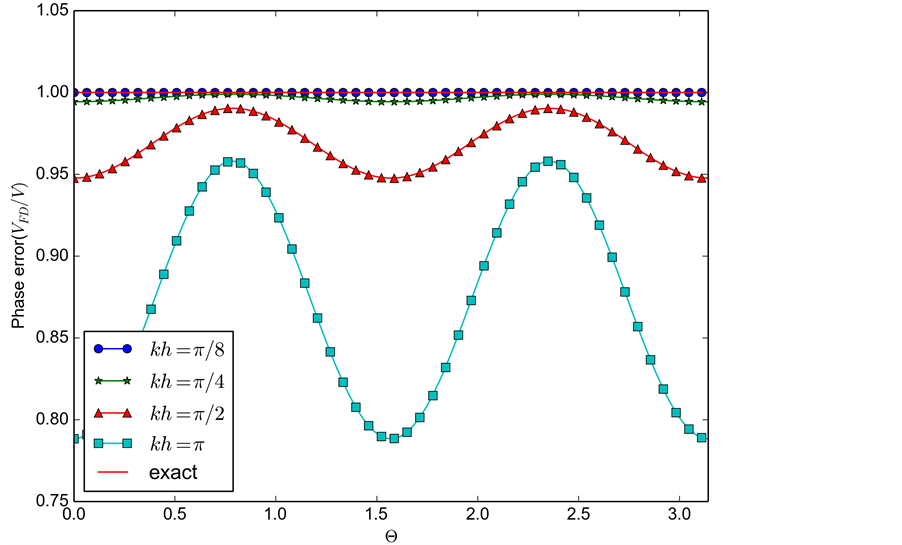
Figure 9. Normalized phase error for different values of kh for CPD-ADI scheme, r = 0.6.

Figure 10. Normalized phase error for different values of kh for NCPD-ADI scheme, r = 0.6.
phase errors, where kh represents polar radius, θ is the polar angle and the plot shows for four values r.
From Figures 13-15 we clearly observe that smaller r values show lower dispersion. It is also shown that waves whose propagation direction makes an angle of 45 degree with the axis are the most accurate for CPD and NCPD schemes, whereas for HOC scheme waves propagating in the axial direction shows relatively low error
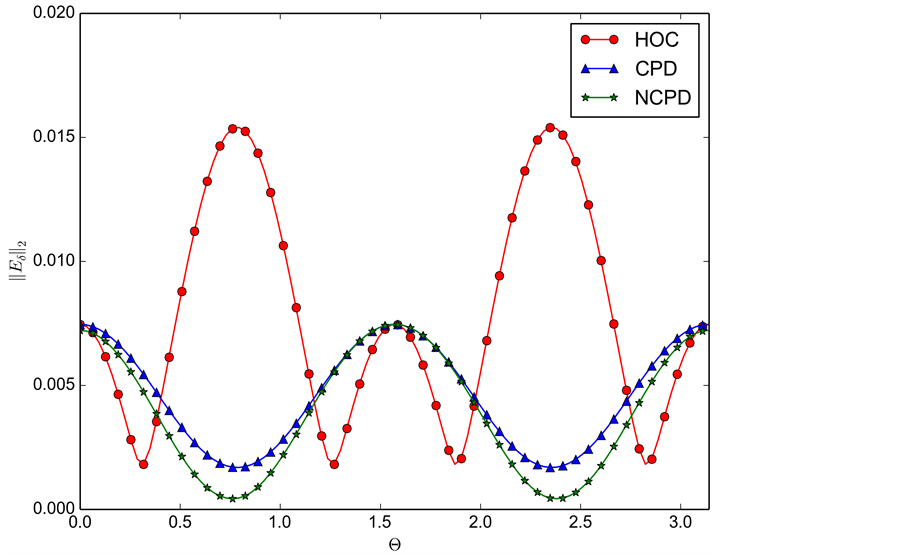
Figure 11. L2-norm of normalized phase error.

Figure 12. Relative phase error for HOC, CPD and NCPD schemes.
for some values of r. Moreover, as clearly indicated, CPD and NCPD schemes show large low dispersion region than HOC scheme.
11. Conclusion
In this thesis, three ADI schemes are presented for 2D and 3D acoustic wave equation with constant velocity. We derived HOC-ADI, CPD-ADI and NCPD-ADI schemes. The former scheme is based on Taylor approximation and the latter schemes are based on Padé approximation. We perform stability analysis for the mentioned
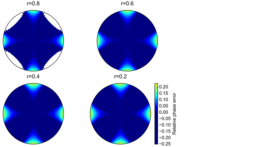
Figure 13. Relative phase error for HOC-ADI scheme for different values of r.
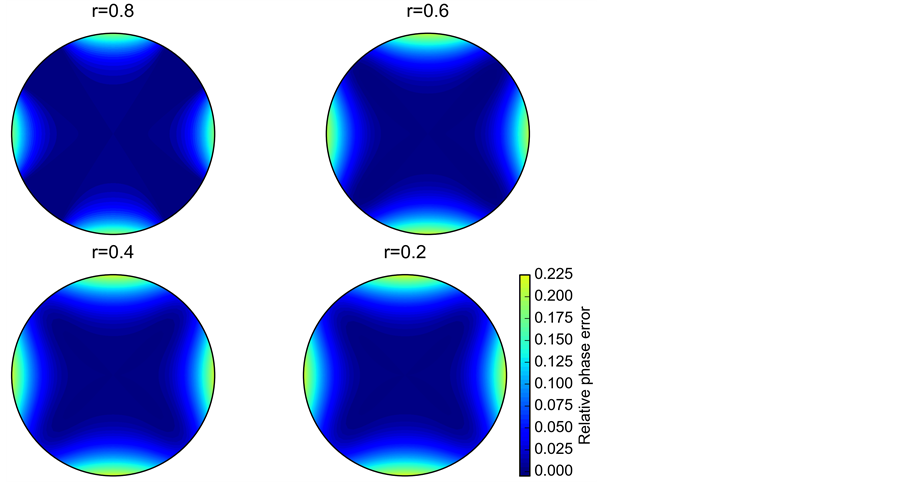
Figure 14. Relative phase error for CPD-ADI scheme for different values of r.

Figure 15. Relative phase error for NCPD-ADI scheme for different values of r.
schemes. Dispersion relations for these schemes have been also obtained followed by a thorough discussion of these relations by plotting them for different parameter sets with respect to different values of kh and θ. From this analysis, it is observed that an increase in these parameters increases the dispersion error and vice-versa. It is observed that numerical dispersion is dependent of these parameters in general for the mentioned schemes.
Comparison of phase errors for these schemes is also carried out with the given parameters. Phase error comparison of the three schemes showed that NCPD scheme has relatively lower dispersion error than CPD and HOC schemes. However, in this work we could only compare dispersion properties for three higher order numerical schemes, therefore in the future, we will analyse dispersion properties of a large group of schemes so that we will be able to explore higher order accurate low dispersive schemes.
Cite this paper
Yahya AliAbdulkadir, (2015) Comparison of Finite Difference Schemes for the Wave Equation Based on Dispersion. Journal of Applied Mathematics and Physics,03,1544-1562. doi: 10.4236/jamp.2015.311179
References
- 1. Canale, R.P. and Chapra, S.C. (1998) Numerical Methods for Engineers with Programming and Software Applications. 3rd Edition, McGraw-Hill, Hoboken.
- 2. Zhou, H.M. (Editor) (2013) Computer Modelling for Injection Modelling Simulation Optimization and Control. John Wiley and Sons, Hoboken.
- 3. Krumpholz, M. and Katehi, L.P.B. (1996) MRTD: New Time-Domain Schemes Based on Multiresolution Analysis. IEEE Transactions on Microwave Theory and Techniques, 44, 555-571.
- 4. Lee, T.-W. and Hagness, S.C. (2004) Pseudospectral Time-Domain Methods for Modeling Optical Wave Propagation in Second-Order Nonlinear Materials. Journal of the Optical Society of America B, 21, 330-342.
http://dx.doi.org/10.1364/JOSAB.21.000330 - 5. Das, S., Liao, W.Y. and Gupta, A. (2013) An Efficient Fourth-Order Low Dispersive Finite Difference Scheme for 2-D Acoustic Wave Equation. Journal of computational and Applied Mathematics, 258, 151-167.
- 6. Liao, W.Y. (2013) On the Dispersion, Stability and Accuracy of a Compact Higher-Order Finite Difference Scheme for 3D Acoustic Wave Equation. Journal of Computational and Applied Mathematics, 270, 571-583.
- 7. Moin, P. (2010) Fundamentals of Engineering Numerical Analysis. 2nd Edition, Cambridge University Press, New York.
http://dx.doi.org/10.1017/CBO9780511781438 - 8. Liu, Y. and Sen, M.K. (2009) Advanced Finite-Difference Methods for Seismic Modeling. Geohorizons, 14, 5-16.
- 9. Smith, G.D. (1985) Numerical Solutions of Partial Differential Equations: Finite Difference Methods. 3rd Edition, Oxford University Press, New York.
- 10. Strikwerda, J.C. (1989) Finite Difference Schemes and Partial Differential Equations. 2nd Edition, Wadsworth and Brooks-Cole.
- 11. Bradie, B. (2006) A Friendly Introduction to Numerical Analysis. Pearson International Edition, Pearson Education Inc., New Jersey.
- 12. Kowalczyk, K. and Van Walstijn, M. (2010) A Comparison of Nonstaggered Compact FDTD Schemes for the 3D Wave Equation. IEEE International Conference on Acoustics Speech and Signal Processing (ICASSP), Dallas, 14-19 March 2010, 197-200.