Modeling and Numerical Simulation of Material Science, 2012, 2, 1-13
http://dx.doi.org/10.4236/mnsms.2012.21001 Published Online January 2012 (http://www.SciRP.org/journal/mnsms)
A Numerical Approach on Reduction of Young’s Modulus
during Deformation of Sheet Metals
Chetan Nikhare
Mechanical Engineering Department, University of New Hampshire, Durham, USA
Received November 23, 2011; revised December 25, 2011; accepted January 3, 2012
ABSTRACT
The paper investigates the elastic behavior of the metal after unloading. For this purpose the strip of metal with tensile
gauge length was simulated with high and low strength material. Further the channel forming was modeled for combi-
nation of materials to predict the spring-back and compared the results. It is observed that the Young’s modulus
(E-value) decreases with the increase in plastic strain. The strength of the material has no effect on the decrease in the
E-value after unloading during tension test. However in channel forming the E-value after unloading depends on the
starting E-value, spring-back angle and maximum strain achieved in the channel. The proposed mathematical equations
to determine the E-value after unloading from the tension test and channel forming test gives very good prediction with
each other. It is also found that the lowest spring-back occurred in the channel with the composite Hard-Soft material.
Keywords: Elasticity; Spring-Back; Channel Forming; Optimization; Deformation
1. Introduction
The shape change of the deformed component after
unloading is called the elastic recovery. This behavior is
been named as the spring-back in sheet metal stamping.
The spring-back is defined in different words by many res-
earchers. The geometrical change in the part after form-
ing when the force from the forming tools was removed
is denotes as spring-back [1]. This behavior is most
common in sheet metal formed components in which the
one or two dimensions are much larger than the other
ones. [1] The dimensional inaccuracy in the stamped part
is due to the spring-back. Some studies shows that the
final shape of the parts depends on the amount of elastic
energy stored in the part during the sheet metal forming
process [2]. The amount of elastic energy stored is a
function of many parameters thus spring-back prediction
is a complicated task. The shape error due to the
spring-back considers as the manufacturing defect in
sheet metal forming process. Another definition of the
spring-back is referred to as the undesirable change of
part shape that occurs upon removal of constraints after
forming [3]. It can be considered a dimensional change
which happens during unloading, due to the occurrence
of primarily elastic recovery of the part.
Spring-back depends on the amount of draw-in during
deformation. More the draw-in, more dominant will be
the spring-back. Other process parameters which tend to
give more spring-back were larger corner radius of the
die set and lower clamping force [4,5]. It has also inves-
tigated that the spring-back also depends on the material
and process parameters. The influencing parameters for
the strong spring-back were in descending order: punch
corner radius, die corner radius, blank holding force, sup-
porting force and lubrication [6]. The study of spring-
back behavior on ultra high strength steel sheet in bend-
ing was performed under controlled condition using CNC
servo press. The spring-back amount measured for the
steel sheets was almost proportional to the ratio of tensile
strength to the elastic modulus. The spring-back was lit-
tle sensitive to the forming speed and the holding time at
the end of the process [7]. Spring-back is a common oc-
currence due to bending of the sheet during forming
whereas curl was observed in the sheet due to material
sliding over the die radius [8]. Curl is also the closest in-
fluential factor for spring-back. The non-linear relation
predicted between curl height and the back tension [8].
This understanding and prediction would not be clear
without the investigation of hardening models.
Some of the numerical studies tried to predict the
spring-back behavior for experimental comparison and
several work-hardening models were evaluated in order
to determine their influence on the numerical prediction
of the spring-back phenomenon [9]. Based on the set of
experimental results the constitutive parameters identifi-
cation was performed [10]. Generally the spring-back
results showed the sensitivity on the work hardening
models. Due to the high level of equivalent plastic strain
achieved in the U-shape channel the differences in the
C
opyright © 2012 SciRes. MNSMS

C. NIKHARE
2
amount of spring-back prediction was not higher [9].
However the differences found in the study [11,12] where
the strain level was quite low compared to the previous
mentioned literature. The study performed [9] on the
work hardening models the differences exist with ex-
perimental comparison and were associated with the pre-
dicted through thickness stress levels. The accurate pre-
diction of the spring-back through the numerical methods
depends on the materials hardening rule [4,5]. The con-
stitutive equation for stress-strain curve for non-linear
combined hardening rule was proposed depend on the
non-linear kinematic hardening theory of Lemaitre and
Chaboche and Barlat89’s yielding function. It was found
that the isotropic hardening rule over predicts the spring-
back behavior compared to the proposed model. It was
also observed that Barlat89’s and Hill48’s yielding func-
tion gave the better co-relation with experiments than the
von-Mises yielding function [13]. This tells that the
spring-back was sensitive to the work-hardening model. In
the forming of U-shape channel it was identified that the
strain path changes and was associated with the bend-
ing-unbending of the channel during forming. It was also
noted that the strain achieved in each strain path are
equally important as the strain path changes during the
forming [9]. It was also shown that one model predicted
larger spring-back angles for some materials and smaller
for other ones according to the predominant strain-paths
and strain-path changes. The comparison on the influ-
ence of the work-hardening models on spring-back, dif-
ferent trends was expected depending on the selected
sheet metal formed part as well as the process conditions
[9]. The numerical prediction of the spring-back was str-
ongly dependent on definition of the constitutive model
for the sheet metal mechanical behaviour under the change
in strain-path and the occurrence of the stress reversal
during the bending to unbending transition on the die
radius [14]. In addition the investigation on number of
integration points through thickness has done by many
researchers to understand the accuracy in prediction [1,
15-20]. Wagoner et al. [21] recommended the implemen-
tation of 25 to 51 IP for 1% accuracy in the prediction.
Previous studies performed on the influence of change
in elasticity during plastic deformation noted quite inter-
esting outcomes found that some simulation results was
in low precision when compared to the experiments [22].
It was found that the E-value varies after plastic defor-
mation [23-29]. Thus consideration of this change in
E-value would be needed to improve the spring-back
simulation. The decrease in E-value was experimentally
shown and proposed the linear relation [29, 30] between
E-value and the plastic strain. The analytical model de-
veloped with the consideration of change in E-value for
the estimation of top roller position predicted larger
spring-back compare to with the constant E-value [24].
Similar results achieved by [26,27] for the U-channel and
predicted closer results with experiments. The micro-
scopic approach through nano-indentation on the indi-
vidual phases showed decrease in E-value with plastic
deformation. Some of the dislocation associated with the
pile-up of dislocations near the grain boundary and was
the influential factor for E-value change [28].
In this study the E-value change was investigated
through the longitudinal tension test and channel forming
model. The tensile gauge sample was deformed for dif-
ferent strain values and the E-value after unloading was
predicted. Further the channel forming was studied for
single material with different starting E-values. The equa-
tion for estimation of E-value after unloading was pro-
posed for both longitudinal tension test and channel
forming model. Both proposed equation were compared
to find the discrepancy in the method. In addition the
channel forming was used to understand the spring-back
behaviour of the composite material. In this different
starting E-value and strength level combination were
simulated.
2. Materials
The materials investigated in this study are the two steel
types for which the tensile true stress-strain curve is
shown in Figure 1 and the mechanical properties are
tabulated in Table 1.
Holloman’s power law (Equation 1) was used to gen-
erate the true stress-strain curve shown in Figure 1.
n σKε (1)
Figure 1. Tensile true stress-strain curve for two steel type
materials.
Table 1. Mechanical properties for the two steel type materials.
Mechanical Properties
Material YS (MPa) K (MPa) n
Soft Metal 183 765 0.23
Hard Metal 359 1500 0.23

C. NIKHARE
3
3. Methodology 3.2. Channel Forming
The elastic behavior of the sample in tension loading and
unloading at different strained condition was simulated
with the longitudinal tension test (Figure 2). Further this
behavior was predicted with the channel forming model
(Figure 3). The spring-back occurred in each case was
predicted and mathematical equations were determined.
In addition the Taguchi method of L9 array was per-
formed to find out the most dominating factor on the
spring-back behavior. Further the combinations of mate-
rials were simulated to understand the effect of different
young’s modulus value and different strength level.
The schematic view of the channel forming model is
shown in Figure 3; was used to form the channels for
spring-back effect. All essential tool dimensions are
mentioned in the Figure 3. For all simulations the
enough blank holder force was applied so that the blank
can slide easily without any stretching. The blank was
used with the length of 85.5 mm and thickness of 2 mm.
The punch depth of 40 mm was applied to all simulation
except for the sensitivity analysis simulations.
3.3. Numerical Method
The longitudinal tension test and channel forming tests
were investigated using ABAQUS/Standard 6.8-1. The
three-dimensional model approach was used for the lon-
gitudinal tension test whereas the two-dimensional model
was used to perform the channel forming test. In longitu-
dinal tension test the reference point was used to apply
the displacement for deformation. The reference point
was constrained to one end of the sample with the help of
coupling constraint. The other end of the tension sample
was fixed. The tension sample was assumed as deform-
able body with C3D8R 8-node linear brick elements.
3.1. Longitudinal Tension Test
The longitudinal test was modeled based on the tensile
sample as recommended in Australian Standard AS
1391-1991 with only the consideration of gauge length of
50mm and gauge width of 12.5 mm on specimens. The
loading-unloading curve for 20 strain values was per-
formed starting from 1% to 20 % strain with the interval
of 1% strain. In each case the unloading E-value was
predicted. In some cases the thickness of the sample was
divided into two sections for the application of different
material properties in each section. Similar procedure
was applied to understand the unloading behavior and the
prediction of E-value.
In channel forming model the tooling was assumed as
rigid surfaces, while for blank deformable CPE4R 4-node
bilinear plane strain elements were applied. Four layers
through the material thickness were used and the maxi-
mum element size was chosen to be 0.5 mm. In the
model the interaction between the blank and the tooling
was assumed with the coefficient of friction of 0.1.
The material curve as shown in Figure 1 with iso-
tropic plasticity was used in all the simulations. The
spring- back measurement is shown in Figure 4. Figure 2. Longitudinal tension tests.
Figure 3. Channel forming model.

C. NIKHARE
4
Figure 4. Spring-back measurement.
3.4. Robust Design
In this section, the Taguchi method was used with an
orthogonal array of L9 to analyse the effect of various
material parameters on the spring-back. The quality
characteristic measured was the spring-back for all the
nine simulations (experiments) designed by the L9 array.
Since the objective is to minimise the spring-back, out of
three signal-to-noise ratios [31] the “smaller the better” is
the option for this study as the aim is to ascertain the
minimum spring-back. The signal-to-noise ratio for
“smaller the better” is given below:

2
10logη θ (2)
The important parameters (control factors) that were
considered and included in the present analysis are:
1) EBD
2) δ
3) K
4) n
Table 2 lists the levels used for the above factors for
channel forming. The chosen numerical values are not
related to any material but comparable to real materials.
The values chosen and set to generate the three levels at
an interval to study the dominating factor which is re-
sponsible for higher springback from the considered four
parameters.
The total number of degrees of freedom for the system
is 9 (two for each of the four control factors and one for the
overall mean). Hence an L9 orthogonal array was chosen to
design the simulation (experiments). The log sheet for the
nine simulations (experiments) is given in Table 3.
4. Results and Discussion
The E-value after unloading at each plastic strain level is
shown in Figure 5. It is found that the E-value decreases
with respect to increase in plastic strain. Three different
Table 2. Control factors and their levels.
Factors Level 1 Level 2 Level 3
EBD 210 130 50
δ 40 30 20
K 1500 1000 500
n 0.25 0.15 0.05
Table 3. Level of control factors for spring-back.
Expt. No.L9 ArrayEBD δ K n
1 1111 210 40 1500 0.25
2 1222 210 30 1000 0.15
3 1333 210 20 500 0.05
4 2123 130 40 1000 0.05
5 2231 130 30 500 0.25
6 2312 130 20 1500 0.15
7 3132 50 40 500 0.15
8 3213 50 30 1500 0.05
9 3321 50 20 1000 0.25
starting E-values (210, 160 and 20 GPa) were modeled
and E-value after unloading was measured for different
level of plastic strain. Based on the curve shown in Fig-
ure 5, the Equation 3 was assumed and proposed to pre-
dict the E-value after unloading with the help of E-value
before loading and the intended plastic strain value. The
calculated E-values after unloading show very good
agreement for all three different curves.
1.5
AD BDBD
EE Eε

 (3)
The spring-back after unloading in channel forming
for 20 different starting E-values (210, 200 till 20) is
shown in Figure 6. The interesting fact is observed that
with the lower starting E-value the curl is more dominant.
Thus it can be noted that for the same strength level the
steel will have significantly lower curl than the alumi-
num and magnesium due to difference in E-value.
The achieved plastic strain after forming and before
spring-back for the maximum strain region (region indi-
cated by square in the inset of Figure 7) is plotted along
the position of elements in the channel (Figure 7). For
same strength level with higher starting E-value the
maximum plastic strain is achieved; whereas for lower
starting E-value the strain value is comparatively very
low. Thus the fact is interesting that the starting E-value
affects the strain level during forming.
The plot of spring-back angle with respect to the
achieved maximum plastic strain for each starting E-
value is shown in Figure 8. The linear relationship is
observed and given in the Equation 4.
1280 156θε

 (4)

C. NIKHARE 5
Figure 5. E-value after unloading at different plastic strain.
Figure 6. Spring-back for different value of initial starting E-
value.
Figure 7. True plastic strain along the channel for a small
section.
Figure 8. Spring-back angle for different starting E-value
with respect to the maximum plastic strain.
The non-linear relation is observed in between the
E-value and the spring-back angle (Figure 9). The rela-
tionship is given in Equation 5. The modified proposed
relationship based on trial and error method understand-
ing and is given in Equation 6 which depends on the
E-value after unloading, spring-back angle and maximum
strain achieved before spring-back. Similarly the non-
linear relation between the E-value after unloading and
the maximum plastic strain achieved before unloading is
shown in Figure 10.
1.126
5502
AD
Eθ  (5)
1.2 ε
AD BD
EEθ

 (6)
4.1. Sensitivity Analysis
The percentage effect of different material parameters are
analysed by performing the nine simulations. The desired

C. NIKHARE
6
and the final profile with spring-back for all 9 simula-
tions are shown in Figure 11. The spring-back angle is
predicted in all nine simulations and tabulated in Table 4.
Here the third setting shows least spring-back as com-
pared to others. This may be due to less punch displace-
ment and softer material.
Fig ure 9. E-value after unloading for their respective spring-
back angle.
Figure 10. E-value after unloading for their respective max-
imum plastic strain.
(a) (b) (c)
(d) (e) (f)
(g) (h) (i)
Figure 11. Spring-back for nine simulations for L9 orthogonal array by Taguchi method.

C. NIKHARE 7
Table 4. Signal-to-noise ratio for nine conditions.
Expt. No. Predicted Spring-back(θ)


2
10log i ηy
1 20.82 –26.37
2 15.76 –23.95
3 8.12 –18.2
4 34.00 –30.63
5 10.31 –20.26
6 17.89 –25.05
7 37.54 –31.49
8 65.89 –36.38
9 21.84 –26.78
Total –239.11
Overall mean –26.357
In Table 5,*value have been used to calculate the
pooled error. The magnitude of variance ratio gives a
measure of the relative contribution of a factor towards
the required minimum pressure, or the sensitivity of the
required pressure for a particular factor. A value of vari-
ance ratio larger than four indicates the effect of a factor to
the quality characteristic is strong, whereas a value less
than one is the indicative of negligible effect. Therefore,
the spring-back is highly sensitive to the E-value before
loading “EBD” and less sensitive to material strain hard-
ening value “n”.
Table 6 shows the average contribution of each factor
which when varied at each level and Figure 12 shows
the graphical plot of this effect. From this it is observed
that the E-value before loading is the most influencing
factor on spring-back. However the contribution of punch
displacement and material strength coefficient is also
much more considerable. The contribution of E-value
before loading is coming 47% whereas the contribution
of punch displacement and material strength coefficient
is almost equal i.e. ~22%.
From the above sensitivity analysis the importance of
E-value before loading, material strength coefficient, mate-
rial strain hardening and the maximum plastic strain attained
in the channel has been understood and the consideration of
these parameters should take in account while determin-
ing the spring-back angle. Thus the Equation (4) is modi-
fied by trial and error method understanding and given in
Equation (7) for single material and Equation (8) for m
number of materials in the composite channel.
5
n
BD
Kε
θE





(7)
12
12
112 2
5
m
m
n nn
mm
BD BDBD
Kε KεKε
θEE E






Table 5. ANOVA for minimum spring-back in channel for-
ming.
Factors Degree
of freedom
Sum
of squares
Mean
square(Vx)
Variance ratio
(F = Vx/Ve)
Percentage
effect
EBD 2 120.9060.45 5.15 47.20%
δ 2 57.30 28.65 2.44 22.36%
K 2 54.5 27.25 2.32 21.26%
n 2 23.48*11.74 1 9.16%
Total8 256.18-- -- --
Pooled
error 2 23.48 11.74
Table 6. Effect at different levels.
Factors Level 1 Level 2 Level 3
EBD –22.84 –25.31 –31.55
δ –29.5 –26.83 –23.34
K –29.26 –27.12 –23.31
n –24.47 –26.83 –28.40
Figure 12. Control factor effect at different levels.
4.2. Different Elasticity Same Strength
Composite Channel



(8)
To understand the composite behavior of E-value change
after unloading, the channel is divided into two sections
similarly as mentioned in the longitudinal tension test.
Each top and bottom layer was given the same hardening
behavior but different starting E-value. Thus four simula-
tions were performed for set of starting E-value 210-200,
210-150, 210-100 and 210-50. Resultant E-value of the
composite was calculated according to the parallel law
[32]. These would be the cases where the composite ma-
terials were generated by joining the two strip materials
e.g. Steel-Aluminum or Steel-Copper etc. The assump-
tion taken while simulating these channels was that the
two strips were perfectly joined together without and
interface defect. The spring-back for all four simulations

C. NIKHARE
8
is shown in Figure 13 and the maximum plastic strain
values for each case are tabulated in Table 7. The pre-
dicted spring-back angle for all four simulations are
tabulated in Table 7 and compared with the calculated
value from Equation 8. The calculated value from the
proposed equation gave the good agreement with the pre-
dicted value. Thus it is noted that the proposed equation
obtain from the single starting E-value analysis can be
applied for the composite of different starting E-values
for comparable results. Similarly the E-value after un-
loading is calculated from equations proposed from the
longitudinal tension test and from channel forming. The
both values are in good co-relation (Table 8).
Figure 13. Spring-back for the combination of E-value with
able 7. Prediction and calculation of spring-back angle for
Combina- Maximum θPrediction
same strength level.
T
different E-value with same strength level.
tions Strain
θMathematical
1
11 2
n
KεK


2
12
2
5
n
BD BD
ε
θEE




210-200 0.1053 21.92 21.79
210-150 0.1021 25.34 25.63
210-100 0.0973 31.54 28.25
210-50 0.0845 47.07 52.18
4.3. Same Elasticity Different Strength
Composite Channel
The behavior of the composite material with different
strength level and same starting E-value was understand
by performing the longitudinal tension test and further
with the channel forming for spring-back. In this section
the channel was assumed as a composite material which
was self generated due to the increase in temperature on
punch or die side during stamping. Due to increase in
temperature the material gets soften and thus difference
in temperature on punch and die side generates the com-
posite strip. This concept probably occurs in stamping
the advanced high strength steel where friction with the
tooling is of more importance. Figure 14 shows the pre-
dicted E-value after unloading at different plastic strain
level for single material; composite material with differ-
ent starting E-value but same strength level and compos-
ite material with same starting E-value but different
strength level. It is found that the prediction for single
material and composite material with same starting E-va-
lue but different strength have same prediction where as
there is no comparison for composite material with dif-
ferent starting E-value but same strength. From this it is
worth to say that strength level does not matter in case
longitudinal test and is completely influence of the start-
ing E-value.
Figure 14. E-value after unloading at different plastic strain.
Table 8. Prediction and calculation of E-value after unloading with same strength level.
Combinations Maximum θMathematical
Strain
12
12
112 2
5
nn
BD BD
KεKε
θEE

 


E
Mathematical
ε
AD
EEθ1.2 BD



E
Mathematical
AD D
Eε  1.5
BD B
E E
210-200 0.1053 21.79 178 172
210-150 0.1021 25.63 155 152
210-100 0.0973 28.25 134 132
210-50 0.0845 52.18 111 113

C. NIKHARE 9
Tstring-back the fobi-
a
n cuts i.e. Sec-
o deeply underand the spur com
ntions of simulation for channel forming were per-
formed i.e. single “Soft” material, composite “Hard-Soft”
material, composite “Soft-Hard” material and single
“Hard” material. In two cases the channel was considered
as only “Soft” material and only “Hard” material. This
implies that there was no increase in temperature during
stamping. In other two cases the channel was considered
as composite material. In these cases the assumption
taken that the increase in temperature during stamping on
the punch and the die side was different and thus makes
the material soft on one side than the other. In one of
these two cases it was assumed that the increase in tem-
perature was higher on the die side and thus the material
named as “Hard-Soft” material. Similarly in the second
case it was assumed that the increase in temperature was
higher on the punch side and thus the material named as
“Soft-Hard” material. All materials were assumed to
have same starting E-value of 210 GPa. It is found that
the predicted profile for single Soft material and compos-
ite of Hard-Soft material are unexpectedly similar (Fig-
ure 15). Whereas the prediction for the single Hard ma-
terial and composite of Soft-Hard material are not
matching with the single soft material spring-back profile
which was expected.
The plastic strain achieved in the channel before spring
back is predicted for the single soft material and the com-
posite Hard-Soft material (Figure 16). It is observed that
the plastic strain achieved at ~35 mm along the channel
(where the bottom bending occurs in the blank) is higher
for composite Hard-Soft material than the single Soft
material. This follows the lower E-value after unloading
in composite Hard-Soft material and expected to get
higher spring-back. Similarly the strain achieved at the
section ~70 mm along the channel (i.e. top bending sec-
tion) are same for both single Soft material and compos-
ite Hard-Soft material and expected to get similar spring-
back. But both expectations were wrong. This may be re-
lated to the different bending mechanism at both top and
bottom corner which is discussed in next section. The pre-
dicted strain and the calculated E-value are plotted for
single Hard material and composite Soft-Hard material
shown in Figures 17 and 18. The maximum strain achie-
ved in all four cases and the corresponding predicted and
calculated spring-back angle and the E-value after un-
loading are tabulated in Tables 9 and 10. It is noted that
the proposed equation can be used to approximately pre-
dict the E-value after unloading and can be use as the
helpful tool to design the die, punch and process.
4.4. Stress Distribution at Corners
In Figure 19 the channel with two sectio
tion I and Section II are shown. In Section I the channel
bent suddenly once the forming process starts whereas in
Section II the channel bend at the end of the forming. In
Figure 15. Spring-back for the combination of strength level
with same E-value.
Figure 16. True plastic strain and E-value after unloading
along the channel for single Soft metal and the composite
Hard-Soft metal.
Figure 17. True plastic strain and E-value after unloading
along the channel for single Hard metal.

C. NIKHARE
10
between the two sections the channel slides continuously
and gives the effect at the end of forming as the cu
Figure 18. True plastic strain and E-value after unloading
along the channel for the composite Soft-Hard metal.
Table 9. Prediction and calculation of spring-back anme E-value.
Combinations Maximum Strain θPrediction θMathematical
rl. In
Section I, the stress levels in both tension and compres-
sion for the single Soft material as well as the composite
Hard-Soft material are almost same (Figure 20) and thus
the spring-back is similar at bottom corner. Whereas the
stress-levels are different in single Hard material and
composite Soft-Hard material. The compression bending
of the hard material was supported by the tension of the
soft material at bottom corner for the composite Hard-Soft
material and thus helped in reduction of the spring-back.
In Section II, the tension as well as the compressive stress
levels for single Soft material is lower than the composite
Hard-Soft material and this is the possible reason to get the
lower spring-back in the later case. The stress levels for
the remaining cases are completely different and thus have
different spring-back (Figure 21).
gle for different strength level with sa
12
12
112 2
5
nn
BD BD
KεKε
θEE

 


Soft 0.1148 13.53 11.07
Hard 0.1057 21.38 21.30
Soft-Hard 0.1161 18.03 15.09
Hard-Soft 0.1228 12.20 15.62
Table 10. Prediction and calculation of E-value after unloading with different strength level.
Combinations Maximum Strain θMathematical
12
12
112 2
5
BD BD
KεKε
θEE 



EMathematical 1.2ε
AD BD
EEθ
nn



 EMathematical AD BD EE1.5BD Eε
Sof148 191 173 t 0.111.07
Hard 0.1057 21.30 182 176
Soft-Hard 0.1161 09 184 173
Hard-Soft 0.1228 15.62 180 171
15.
5. Conc
The E-value a
simple longitud
test. It was found that the E-value after unloading de-
chla. It was also ob-
served that the E-value after unloading in longitudinal ten-
sion epends oarting E-value and has no effect
of st level oaterial. Further ring-back
prediwas studith the channel fodel.
Heion osed to determe E-value
afting wpends on the st E-value,
ring-back angle and the maximum strain value achieved
proposed equation for E-value with
nsion test and channel forming model
gave the similar prediction and can be used as the tool to
lusions
fter unloading was performed with the
inal tension test and the channel forming
reases with te increase in pstic strain
test dn the st
rength
ction
f the m
ed wi
the sp
orming m
re the equatwas propine th
er unloadhich dearting
sp
in the channel. The
both longitudinal te
Figure 19. Two sections of channel for stress analysis.

C. NIKHARE 11
(a) (b) (c) (d)
Figure 20. Stress level achieved at Section I by compression and tension loading for (a) Soft, (b) Hard-Soft, (c) Soft-Hard, (d)
Hard metal.
(a) (b) (c) (d)
Figure 21. Stress level achieved at Section II by compression and tension loading for (a) Soft, (b) Hard-Soft, (c) Soft-Hard, (d)
Hard metal.
design the die, punch and the process to reduce the
spring-back. In addition the spring-back prediction was
studied for the composite material. The interesting fact
was observed that the stress level in both tension and
compression are same in both single Soft material and
composite Hard-Soft material and thus gave the similar
amount of spring-back prediction. Therefore this can be
use as a helpful tool to design the new material for the
elimination of spring-back. This indicated that the com-
posite material with Hard layer touches to punch and soft
layer touches to the die will give the same spring-back
for the single softer material.
6. Acknowledgements
The author would like to extend his gratitude to Professor
Peter D. Hodgson and Professor Brad L. Kinsey for sup-
port and Deakin University and University of New Ham-
pshire for providing the facility to carry out this research
work.

C. NIKHARE
12
REFERENCES
[1] R. Wagoner and M. Li, “Simulation of Springback: Through-
Thickness Integration,” International Journal of Plastic-
ity, Vol. 23, No. 3, 2007, pp. 345-360.
doi:10.1016/j.ijplas.2006.04.005
[2] N. Narasimhan and M. Lovell, “Predicting Springback in
Sheet Metal Forming: An Explicit to Implicit Sequential
Solution Procedure,” Finite Elements in Analysis and De-
sign, Vol. 33, No. 1, 1999, pp. 29-42.
doi:10.1016/S0168-874X(99)00009-8
[3] H. S. Cheng, J. Cao and Z. Xia, “An Accelerated Spring-
back Compensation Method,” International Journal of
Mechanical Sciences, Vol. 49, No. 3, 2007, pp. 267-279.
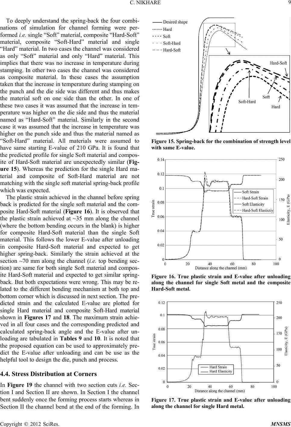
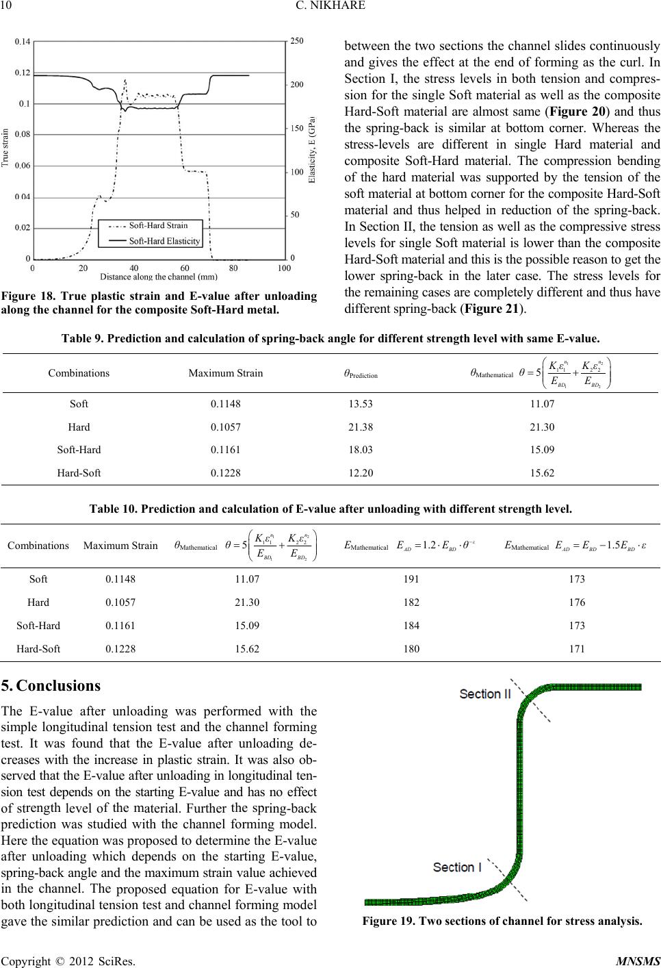
doi:10.1016/j.ijmecsci.2006.09.008
[4] K. Li, W. Carden and R. Wagoner, “Simulation of Spring-
back,” International Journal of Mechanical Sciences, Vol.
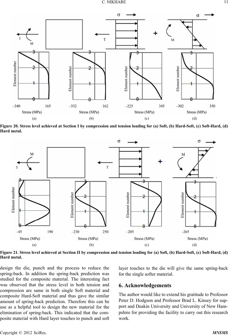
44, No. 1, 2002, pp. 103-122.
doi:10.1016/S0020-7403(01)00083-2
[5] J. Gau and G. Kinzel, “A New Model for Springback
Prediction i
016/S0020-7403(01)00012-1
n which the Bauschinger Effect Is Consid-
ered,” International Journal of Mechanical Sciences, Vol.
43, No. 8, 2001, pp. 1813-1832.
doi:10.1
[6] S. Lee and Y. Kim, “A Study on the Springback in the
Sheet Metal Flange Drawing,” Journal of Materials
Processing Technology, Vol. 187-188, 2007, pp. 89-93.
doi:10.1016/j.jmatprotec.2006.11.079
[7] K. Mori, K. Akita and Y. Abe, “Springback Behaviour in
Bending of Ultra-High-Strength Steel Sheets Using CNC
Servo Press,” International Journal of Machine Tools and
Manufacture, Vol. 47, No. 2, 2007, pp. 321-325.
doi:10.1016/j.ijmachtools.2006.03.013
[8] T. Hilditch, J. Speer and D. Matlock, “Influence of
Low-Strain Deformation Characteristics of High Strength
Sheet Steel on Curl and Springback in Bend-Under-Ten-
sion Tests,” Journal of Materials Processing Technology,
Vol. 182, No. 1-3, 2007, pp. 84-94.
006.06.020doi:10.1016/j.jmatprotec.2
. M. Chaparro and L. F. Me-[9] M. Oliveira, J. L. Alves, B
nezes, “Study on the Influence of Work-Hardening Mod-
eling in Springback Prediction,” International Journal of
Plasticity, Vol. 23, No. 3, 2007, pp. 516-543.
doi:10.1016/j.ijplas.2006.07.003
[10] H. Haddadi, S. Bouvier, M. Banu, C. Maier and C. Teo-
dosiu, “Towards an Accurate Description of the Anisot-
ropic Behaviour of Sheet Metals under Large Plastic De-
formations: Malysis and Identifi-
cation,” Intern ticity, Vol. 22, No.
odelling, Numerical An
ational Journal of Plas
12, 2006, pp. 2226-2271.
doi:10.1016/j.ijplas.2006.03.010
[11] B. M. Chaparro, M. C. Oliveira, J. L. A
nezes, “Work Hardening Models
lves and L. F. Me-
and the Numerica l Si-
mulation of the Deep Drawing Process,” Material Science
Forum, Vol. 455-456, 2004, pp. 717-722.
doi:10.4028/www.scientific.net/MSF.455-456.717
[12] S. Bouvier, J. L. Alves, M. C. Oliveira and L. F. Menezes,
“Modelling of Anisotropic Work-Harde ning Behaviour
Computational Materials Science, Vol. 32, No. 3-4, 2005,
pp. 301-315. doi:10.1016/j.commatsci.2004.09.038
[13] Z. Dongjuan, C. Zhenshan, R. Xueyu and L. Yuqiang,
“Sheet Springback Prediction Based on Non-Linear Com-
bined Hardening Rule and Barlat89’s Yielding Function,”
Computational Materials Science, Vol. 38, No. 2, 2006,
pp. 256-262. doi:10.1016/j.commatsci.2006.02.007
[14] J. Alves, M. Oliveira and L. Menezes, “Drawbeads: To
Be or Not To Be,” In: J. Cao, et al., Editors, Numi-
sheet ’05 6th International Conference and Workshop on
Numerical Simulation of 3D Sheet Forming Processes:
On the Cutting Edge of Technology, Part A, The Ameri-
can Institute of Physics 778, NUMISHEET 2005 Con-
ference, 15-19 August 2005, Detroit, Michigan, pp. 655-
660.
[15] A. Andersson and S. Holmberg, “Simulation and Verifi-
cation of Different Parameters Effect on Springback Re-
sults,” NUMISHEET, Jeju Island, Korea, 21-25 October
2002, pp. 201-206.
[16] N. Yamamura, T. Kuwabara and A. Makinouchi, “Spring-
d Drawbending
MISHEET, Jeju Island, Korea, 21-25 October 2002, pp.
ing—Anisotropy Ef-
“Techniques to Im-
homson, “Prediction of
etals,” Proceedings
. Feng, “Sensitive
of
Metallic Materials Subjected to Strain-Path Changes,”
back Simulations for Stretch-Bending an
Processes Using the Static Explicit FEM Code, with an
Algorithm for Canceling Non-Equilibrated Forces,” NU-
25-30.
[17] L. Bjorkhaug and T. Welo, “Local Calibration of Alumi-
num Profiles in Rotary Stretch Bend
fects,” Materials Processes and Design: Modeling, Simu-
lation and Applications, NUMIFORM, Columbus, OH,
USA, 2004, pp. 749-754.
[18] H. Yao, S. D. Liu, C. Du and Y. Hu,
prove Springback Prediction Accuracy Using Dynamic
Explicit FEA Codes,” SAE TRANSACTIONS, Vol. 111,
2002, pp. 100-106.
[19] V. Nguyen, Z. Chen and P. T
Spring-Back in Anisotropic Sheet M
of the Institution of Mechanical Engineers, Part C: Jour-
nal of Mechanical Engineering Science, Vol. 218, No. 6,
2004, pp. 651-661.
[20] W. Xu, C. H. Ma, C. H. Li and W. J
Factors in Springback Simulation for Sheet Metal Form-
ing,” Journal of Materials Processing Technology, Vol.
151, No. 1-3, 2004, pp. 217-222.
doi:10.1016/j.jmatprotec.2004.04.044
[21] R. Wagoner, L. Geng and K. Li, “Simulation of Spring-
udin, “Experimental
back of High-Per-
in Finite
,” Computers & Struc-
back with the Draw/Bend Test,” IPMM ’99: The Second
International Conference on Intelligent Processing and
Manufacturing of Materials, Honolulu, HI, USA, 10-15
July 1999, pp. 91-104.
[22] C. Hinsinger, V. Zwilling and O. H
and Numerical Approaches of Spring
formance Steels Drawn With U-Shaped Tools and An
Industrial Side Member Tool,” SAE TRANSACTIONS,
Vol. 111, 2002, pp. 2054-2068.
[23] S. Chatti, “Effect of the Elasticity Formulation
Strain on Springback Prediction
tures, Vol. 88, No. 11-12, 2010, pp. 796-805.
doi:10.1016/j.compstruc.2010.03.005

C. NIKHARE
13
on, Chicago, IL, USA, 5-10
197
[24] A. Gandhi and H. Raval, “Analytical Modeling of Top
Roller Position for Multiple Pass (3-Roller) Cylindrical
Forming of Plates,” International Mechanical Engineer-
ing Congress and Expositi
November 2006, pp. 107-116.
[25] A. Gandhi and H. Raval, “Analytical and Empirical Mod-
eling of Top Roller Position for Three-Roller Cylindrical
Bending of Plates and Its Experimental Verification,”
Journal of Materials Processing Technology, Vol.
No. 1-3, 2008, pp. 268-278.
,
doi:10.1016/j.jmatprotec.2007.06.033
[26] H. Yu, “Variation of Elastic Modulus during Plastic De-
formation and Its Influence on Springback,” Materials &
Design, Vol. 30, No. 3, 2009, pp. 846-850.
doi:10.1016/j.matdes.2008.05.064
[27] F. Morestin and M. Boivin, “On the Necessity of Taking
into Account the Variation in the Young Modulus with
Plastic Strain in Elastic-Plastic Software,” Nuclear Engi-
neering and Design, Vol. 162, No. 1, 1996, pp. 107-116.
doi:10.1016/0029-5493(95)01123-4
[28] M. Yang, Y. Akiyama and T. Sasaki, “Evaluation of
Change in Material Properties Due to Plastic Deforma-
tion,” Journal of Materials Processing Technology, Vol.
151, No. 1-3, 2004, pp. 232-236.
doi:10.1016/j.jmatprotec.2004.04.114
[29] D. Fei and P. Hodgson, “Experimental and Numerical
Studies of Springback in Air V-Bending Process for Cold
Rolled TRIP Steels,” Nuclear Engineering and Design,
Vol. 236, No. 18, 2006, pp. 1847-1851.
doi:10.1016/j.nucengdes.2006.01.016
[30] F. Yoshida, T. Uemori and K. Fujiwara, “Elastic-Plastic
Behavior of Steel Sheets under In-Plane Cyclic Ten-
sion-Compression at Large Strain,” International Journal
of Plasticity, Vol. 18, 2002, pp. 633-659.
doi:10.1016/S0749-6419(01)00049-3
[31] M. Phadke, “Quality Engineering Using Robust Design,”
Prentice Hall, Englewood Cliffs, NJ, USA, 1989.
[32] R. Hibbeler, “Mechanics of Materials,” 7th Edition, Pear-
son Education, Cranbury, NJ, USA, 2008.
2……m indicates for material 1, 2……m in
or before loading or
Nomenclature
E-value—Material Young’s modulus
YS—Material Yield Strength
σ—True stress
ε—True plastic strain (In case of subscript 1, 2……m
indicates for material 1, 2……m in composite material)
K—Material strength coefficient (In case of subscript
1, 2……m indicates for material 1, 2……m in composite
material)
n—Material strain hardening exponent (In case of
subscript 1,
composite material)
η—Optimise function for sensitivity analysis
θ—Spring-back angle or Theta
EBD—E-value before deformation
starting E-value (In case of subscript 1, 2……m indicates
for material 1, 2……m in composite material)
EAD—E-value after deformation or after unloading
δ: Punch displacement in channel forming
ft-Hard material—The composSo ite material which
has the soft layer touches the punch and hard layer
touches the die