Applied Mathematics, 2011, 2, 1497-1506
doi:10.4236/am.2011.212212 Published Online December 2011 (http://www.SciRP.org/journal/am)
Precision of a Parabolic Optimum Calculated from Noisy
Biological Data, and Implications for Quantitative
Optimization of Biventricular Pacemakers
(Cardiac Resynchronization Therapy)
Darrel P. Francis
International Centre for Circulatory Health, National Heart and Lung Institute,
Imperial College London, London, United Kingdom
Received August 26, 2011; revised November 9, 2011; accepted November 17, 2011
Abstract
In patients with heart failure and disordered intracardiac conduction of activation, doctors implant a biven-
tricular pacemaker (“cardiac resynchronization therapy”, CRT) to allow adjustment of the relative timings of
activation of parts of the heart. The process of selecting the pacemaker timings that maximize cardiac func-
tion is called “optimization”. Although optimization—more than any other clinical assessment—needs to be
precise, it is not yet conventional to report the standard error of the optimum alongside its value in clinical
practice, nor even in research, because no method is available to calculate precision from one optimization
dataset. Moreover, as long as the determinants of precision remain unknown, they will remain unconsidered,
preventing candidate haemodynamic variables from being screened for suitability for use in optimization.
This manuscript derives algebraically a clinically-applicable method to calculate the precision of the opti-
mum value of x arising from fitting noisy biological measurements of y (such as blood flow or pressure) ob-
tained at a series of known values of x (such as atrioventricular or interventricular delay) to a quadratic curve.
A formula for uncertainty in the optimum value of x is obtained, in terms of the amount of scatter (irrepro-
ducibility) of y, the intensity of its curvature with respect to x, the width of the range and number of values of
x tested, the number of replicate measurements made at each value of x, and the position of the optimum
within the tested range. The ratio of scatter to curvature is found to be the overwhelming practical determi-
nant of precision of the optimum. The new formulae have three uses. First, they are a basic science for any-
one desiring time-efficient, reliable optimization protocols. Second, asking for the precision of every re-
ported optimum may expose optimization methods whose precision is unacceptable. Third, evaluating preci-
sion quantitatively will help clinicians decide whether an apparent change in optimum between successive
visits is real and not just noise.
Keywords: Cardiac, Pacemaker, Parabolic, Haemodynamics
1. Introduction
Plato, Apology of Socrates, 38a
Every year, ~100,000 cardiac resynchronization pace-
makers are being implanted into patients with heart fail-
ure, because they deliver substantial symptomatic and
survival benefits [1-3] by altering intracardiac timings.
After implantation, the process of determining which ti-
mings to programme is described as “optimization” [4-6].
Responses of physiological variables to changes in pace-
maker settings fit well to a parabola in the vicinity of the
optimum [6,7]. Curve-fitting to calculate a clinical opti-
mum has the advantage of permitting interpolation to
settings which were not directly tested, and also avoids
the problem that simply “picking the highest” leads to
illusory optima, illusory increments in physiology from
optimization, and illusory changes in optimum over time
[8].
In clinical practice physiological measurements con-

D. P. FRANCIS 1498
tain noise which can sometimes be substantial in com-
parison to the underlying signal, and which prevents the
true underlying optimum being identified precisely even
with curve fitting (Figure 1). The impact of such noise
can be reduced by averaging multiple measurements, but
this consumes resources such as time in a clinical envi-
ronment or battery power if the measurements are con-
ducted by the implanted device. It is therefore important
to be able to calculate the precision of an optimum so
that resource usage can be planned to be appropriate to
achieve the clinically-required precision.
As well as needing to know how many replicates are
required, doctors planning an optimization protocol also
need guidance regarding what range of settings to cover
during testing, and how coarsely or finely. Widening the
range or making finer-grained measurements (i.e. at
more closely-spaced intervals) increase the cost of the
optimization process, and so are only justified if there is
a clinically-valuable increase in precision of the opti-
mum.
Finally, doctors caring for patients from day to day
need to know the uncertainty of the optimum obtained
this clinical optimization process. Without this know-
ledge, it is impossible to interpret apparent differences in
optimum within an individual patient between one as-
sessment method and another, or over time [8,9] or after
an operation or a heart attack.
This paper derives a simple formula for the uncer-
tainty of the parabolically-defined optimal setting of a
pacemaker, and presents practical implications for pro-
tocol design and for medical practice.
2. Description of Method
2.1. Physiological Measurements with Noise
The pacemaker setting may be adjusted over a wide ran-
ge of values. Within individual patients, clinical infor-
mation provides a priori a constrained range which con-
tains all biologically plausible locations of the optimum
for that patient. During the optimization procedure, the
clinician acquires a series of pairs of values of the pace-
maker setting and the corresponding physiological mea-
surement. The first value, the pacemaker setting, has
negligible uncertainty because it is programmed digitally.
However the second value, the measured physiological
variable, is not perfectly reproducible and therefore has
an element of uncertainty.
Some choices of physiological variable, such as blood
pressure, permit automatic acquisition, while others, such
as Doppler velocity-time integral, typically require hu-
man involvement for each measurement. In practice the
protocol is often to make more than one replicate mea-
surement at each setting, and then to summarize the data
80100 120 140 160
90
100
110
1
111
12
2
2
2
2
3
3
3
3
3
1
111
1
2
2
2
2
2
3
333
3
Optimization
#1
Optimization
#2
Optimization
#3
Three
optimization
datas ets
Three
clinical
optima
Uncer tainty
in location
of optimum
AV delay (ms)
Physiological
response
(arbitrary units)
80100 120 140 160
90
100
110
1
111
12
2
2
2
2
3
3
3
3
3
1
111
1
2
2
2
2
2
3
333
3
Optimization
#1
Optimization
#2
Optimization
#3
Three
optimization
datas ets
Three
clinical
optima
Uncer tainty
in location
of optimum
AV delay (ms)
Physiological
response
(arbitrary units)
Figure 1. Sketch showing how noise in the measured data
creates uncertainty in the optimum. Note: If there is enough
time to conduct many optimizations, they can be analyzed
separately to provide separ ate estimates of the optimum, so
the uncertainty in the optimum can be observed. The upper
panel sketches 3 optimization datasets in one simulated
patient. All 3 datasets are plotted on the same graph and
labeled “1” to “3”. The lower panel shows the 3 individual
interpolated optima obtained by curve fitting with a parab-
ola. This paper provides a method of calculating the uncer-
tainty in a clinically-obtained optimum, without having to
conduct several indepe nde nt optimizations.
for each setting by the mean of the raw measurements at
that setting.
Let the optimization protocol try S different values xi
of the pacemaker setting, evenly spaced at intervals of x.
Let the averaged physiological measurements represent-
ing each setting be denoted yi, each of which is the mean
of R replicate raw measurements. The observed data yi
during clinical testing are composed of an underlying
value yund,i and an error component εR.
,und R ii
yy



Let us consider the error component to be independent

D. P. FRANCIS1499
of yund,i and normally distributed, with its standard devia-
tion for a single raw measurement being 1


and, by
the central limit theorem, the standard deviation for the
error εR of the average of R replicates being
1R

R  .
2.2. The Optimization Process
The best-fit parabola, Axi
2 + Bxi + C, to the observed data
is defined by the standard least-squares method, to
minimize the squared deviation between the observations
yi and the parabola. The clinical optimum from that fitted
parabola is –B/2A, which will differ from the true opti-
mum OptTrue by an amount whose standard deviation can
be calculated as follows. The best-fit parabola is defined
by having A, B and C values that minimize the squared
error

2
2
ii i
F
AxBxC y
.
This is achieved by setting all the partial derivatives of
F with respect to A, B and C to zero:



22
2
2
20
20
20
ii ii
ii i
ii i
FAAxBxCyx
FBAxBxCyx
i
F CAxBxCy

 


 



 




2
ii
ii
i

Therefore
432
32
21
iii
iii
ii
A
xBxCx xy
A
xBxCxxy
A
xBxCy
 





These can be solved for A, B and C as follows:


22
2
42
42
22
42
,
iii i
ii
iiiiiii
iii
Sxyx y
A
Sx x
2
x
yxyx
BC
xSx x








xy
3. Results
3.1. The Clinical Optimum
The clinician will choose as optimal the pacemaker set-
ting which corresponds to the middle of the fitted parab-
ola, i.e. ˆ2
opt
B
x
A

. In terms of the clinical data xi and yi,
this clinical optimum is

2
24
22 2
ˆ22
ii
opt
iii i
xSx
xSx xyxy



 
For simplicity, and without loss of generality, a coor-
dinate system for x can be chosen that makes 0 the centre
of the range of settings tested during optimization. This
symmetrical arrangement of xi values provides the fol-
lowing convenient identities:

 



22
344 2
0,11 12,
0,1 371 240
ii
ii
xxxSSS
xxxSSSS





Applying these substitutions permits the clinical opti-
mum to be described as follows:



22
22 2
24
ˆ
51 60
ii
opt
ii
Sxxy
xSxy x

 


i
y
. (1)
If yi is augmented by any constant k, the numerator is
unchanged because


iiiii ii
x
ykxykx xy 


. The denomi-
nator is also unchanged because it is augmented by


22 2
51 60
i
Sxkkx 



which is


22
22
60 1
51 12
kxSS
kS Sx 0

 .
Therefore without loss of generality the observed val-
ues yi may be defined in terms of the underlying quad-
ratic curvature coefficient Aund, the true optimum xopt, and
the noise component εR as follows:


2
,iundioptR i
yA xx





2
,
22
,
2
22
,
2
1
12
iundioptRi
undioptioptR i
undundoptR i
yAxx
AxxxSx
SS
Ax ASx








 






2
,
322
,
2
2
,
2
1
6
iiiundioptRi
undiopt iopt iiRi
optundiR i
xyxAxx
Axxxxxx
SS
xA xx











 




 
2
22
,
43222
,
22 2
422
2
,
2
13 71
240 12
iiiundioptR i
undiopt ioptiiRi
und opt
iRi
xyx Axx
Axxxxx x
SS SSS
Ax xx
x












 


 








3.2. Expression for the Clinical Optimum
i
.
Applying these within Equation (1) gives:

D. P. FRANCIS 1500
 
   
 
2
22 2
,
222
22 224222
, ,
2
222
,
ˆ
1
24 6
1137
51 60
12240 12
1
24 212
opt
optundiRi
undundoptR iundoptiR i
optundiRi
x
SS
SxxAx x
SSSS SSS
SxAx ASxAxxxx
SS
SxxAxx







 







 






 






 
2
1





 
 

  
222
22 242
,,
22
422
,
222222
44 2
,,
1137
5 16060
12 240
14
24
3
51 11375160
12 4
undR iundiR i
undoptiR i
Rii Ri
und und
SSSS S
S xAxAxx
SS S
Ax xSxx
SSSSSSS x
xx x
AA














 
 









 

  
222 2
4
,
222 2
4 2
,,
,
22
2
,,
2242 2
1424
3
ˆ
1451 60
3
6
1
15 180
141
optiR i
und
opt
Rii Ri
und und
optiRi
und
4
R
ii
und und
SS SSx
xx x
A
xSS SSx
xx
AA
xx
AxSS
x
A xSSA xSSS



Ri


 
 
 
 



 




3.3. Imprecision of the Clinical Optimum
It can be seen from this that the clinically observed opti-
mum ˆopt
x
differs from the underlying optimum opt
x
because of two types of error, which affect the numerator
and denominator respectively. The component in the
numerator is a simple additive error. The impact of the
denominator error, however, scales with opt
x
.
In clinical situations where the errors are large in com-
parison with the degree of curvature that is manifested,
the entire denominator of this formula falls near (or be-
yond) zero and behavior of the expression becomes
strongly nonlinear. In such a situation there is almost no
useful information about the underlying optimum avai-
lable from the acquired data. Clinically this can be con-
sidered likely whenever the information content (or in-
traclass correlation coefficient) is low [8].
In most situations of well-designed optimization pro-
tocols, however, the error is not large compared with the
curvature of the signal, which makes it possible to pro-
vide a closed-form expression for the imprecision of the
optimum.
To do this, the variance of the numerator is first shown
to be

 
,
22
1
2
222
22 222
1
2
6
1
63
11
R
R
iRi
und
S
S
und und
i
Var x
AxSS
i
AxSSA xSS

















 



Likewise the variance of the denominator is

 

 
 
,
22
2
,
42 2
22
,
22 2
2
24 22
15
4
180
14
151 12
14
180
14
R
Ri
und
iRi
und
Ri
und
und
Var AxSS
x
AxSS S
Si
Var AxSS S
AxSS S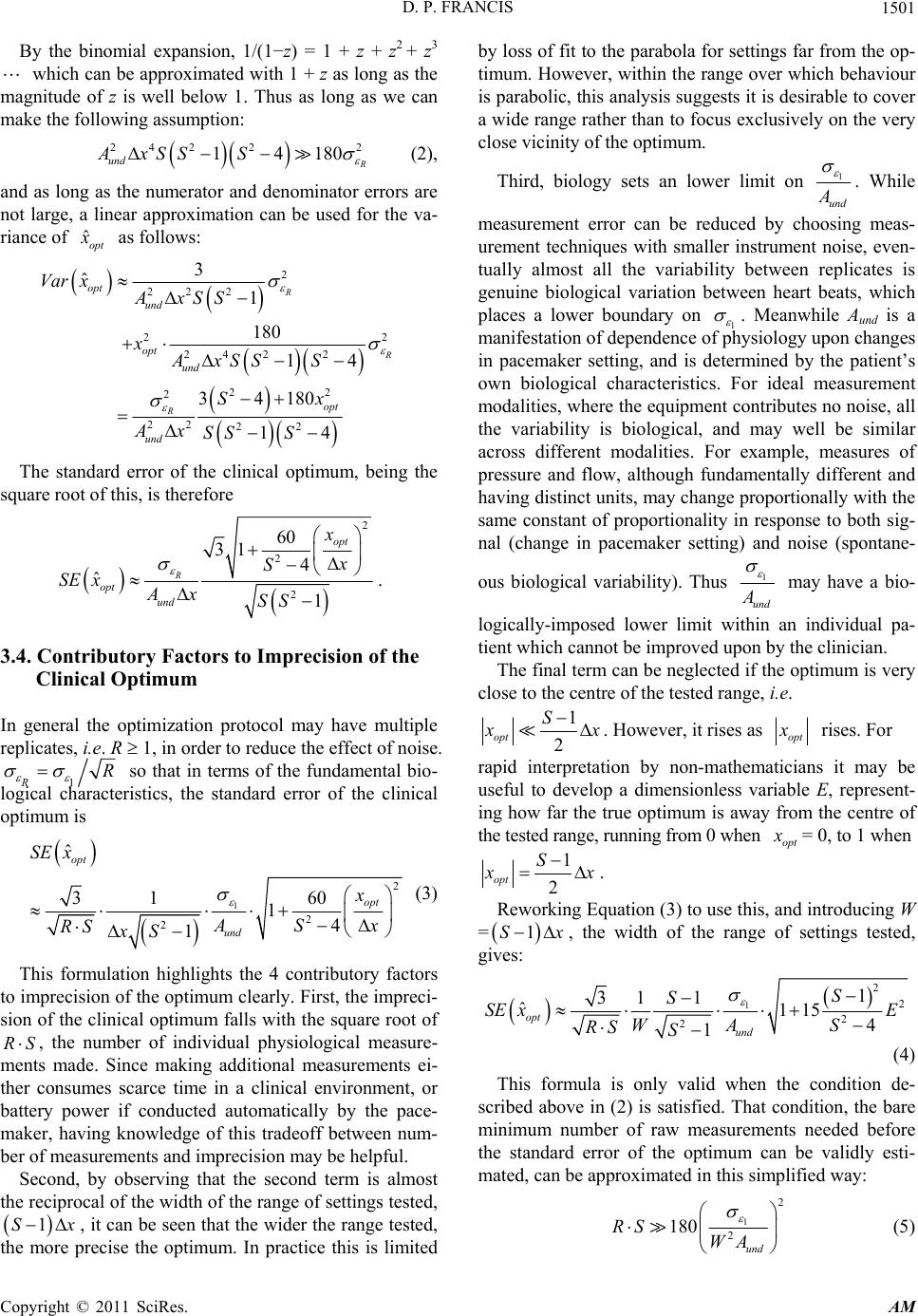































D. P. FRANCIS1501
By the binomial expansion, 1/(1−z) = 1 + z + z2 + z3
which can be approximated with 1 + z as long as the
magnitude of z is well below 1. Thus as long as we can
make the following assumption:




24 222
14180
R
und
AxSS S


 (2),
and as long as the numerator and denominator errors are
not large, a linear approximation can be used for the va-
riance of ˆopt
x
as follows:


 

 
2
22 2
2
24 22
22
2
22 22
3
ˆ
1
180
14
34180
14
R
2
R
R
opt
und
opt
und
opt
und
Var xAxSS
xAxSS S
Sx
Ax
SS S







 


The standard error of the clinical optimum, being the
square root of this, is therefore


2
2
2
60
31 4
ˆ
1
R
opt
opt
und
x
x S
SE xAx SS




 
.
3.4. Contributory Factors to Imprecision of the
Clinical Optimum
In general the optimization protocol may have multiple
replicates, i.e. R  1, in order to reduce the effect of noise.
1R

so that in terms of the fundamental bio-
logical characteristics, the standard error of the clinical
optimum is
R  



1
2
2
2
ˆ
31 60
14
1
opt
opt
und
SE x
x
A
x S
RS xS



 





(3)
This formulation highlights the 4 contributory factors
to imprecision of the optimum clearly. First, the impreci-
sion of the clinical optimum falls with the square root of
, the number of individual physiological measure-
ments made. Since making additional measurements ei-
ther consumes scarce time in a clinical environment, or
battery power if conducted automatically by the pace-
maker, having knowledge of this tradeoff between num-
ber of measurements and imprecision may be helpful.
SR 
Second, by observing that the second term is almost
the reciprocal of the width of the range of settings tested,
, it can be seen that the wider the range tested,
the more precise the optimum. In practice this is limited
by loss of fit to the parabola for settings far from the op-
timum. However, within the range over which behaviour
is parabolic, this analysis suggests it is desirable to cover
a wide range rather than to focus exclusively on the very
close vicinity of the optimum.

1S
Third, biology sets an lower limit on 1
und
A


. While
measurement error can be reduced by choosing meas-
urement techniques with smaller instrument noise, even-
tually almost all the variability between replicates is
genuine biological variation between heart beats, which
places a lower boundary on 1


. Meanwhile Aund is a
manifestation of dependence of physiology upon changes
in pacemaker setting, and is determined by the patient’s
own biological characteristics. For ideal measurement
modalities, where the equipment contributes no noise, all
the variability is biological, and may well be similar
across different modalities. For example, measures of
pressure and flow, although fundamentally different and
having distinct units, may change proportionally with the
same constant of proportionality in response to both sig-
nal (change in pacemaker setting) and noise (spontane-
ous biological variability). Thus 1
und
A


may have a bio-
logically-imposed lower limit within an individual pa-
tient which cannot be improved upon by the clinician.
The final term can be neglected if the optimum is very
close to the centre of the tested range, i.e.
1
2
opt
S
x
x


. However, it rises as opt
x
rises. For
rapid interpretation by non-mathematicians it may be
useful to develop a dimensionless variable E, represent-
ing how far the true optimum is away from the centre of
the tested range, running from 0 when opt
x
= 0, to 1 when
1
2
opt
S
x
x


.
Reworking Equation (3) to use this, and introducing W
=


1Sx

, the width of the range of settings tested,
gives:


1
2
2
2
2
1
31 1
ˆ1154
1
opt
und
S
S
SE xE
WA S
RS S




 


(4)
This formula is only valid when the condition de-
scribed above in (2) is satisfied. That condition, the bare
minimum number of raw measurements needed before
the standard error of the optimum can be validly esti-
mated, can be approximated in this simplified way:
1
2
2
180
und
RS WA






x
(5)

D. P. FRANCIS 1502
If exceeds the above formula by (for example)
more than 5-fold, the uncertainty of the optimum is iden-
tified reliably using Equation (4). If exceeds by
only a small margin, Equation (4) will underestimate the
observed scatter between repeat optimizations. Finally, if
R
 S does not even exceed the right hand side, the dataset
is so poor in information content that it should be dis-
carded, and the protocol redesigned.
RS
RS
In practice the doctor does not know the underlying
values of 1


and und
A
but instead assesses them from
clinical measurements: 1 ˆ


and ˆ
A
respectively.
Figure 2 summarizes all the relevant variables in a
format convenient for visual appreciation. It shows the
steps necessary to gauge the uncertainty of the optimum.
The expressions can be applied to any unit of “pace-
maker setting”, and any unit of “physiological response”.
Typically pacemaker settings (atrioventricular and inter-
ventricular delay) are expressed in either milliseconds or
seconds. Physiological response may be based on flow,
for which suitable units might be true flow rates (e.g.
ml/min, L/min) or expressed per beat (ml/beat), or as a
peak instantaneous flow rate, or as an average velocity
(cm/min or m/min) or peak velocity, or velocity-time
integral (cm/beat). Alternatively physiological response
may be pressure (e.g. mmHg) as a systolic, mean, or
pulse pressure, or a value derived from pressure such as
intraventricular peak first derivative of pressure (dp/dtmax).
In principle uncalibrated physiological response vari-
ables and even those of unknown physical unit may be
used, as long as it is reasonable to believe they vary ap-
proximately linearly with cardiac performance.
Any physical units may be used to express scatter 1


and width W but, once they are decided, the units that
must be used to express curvature und
A
are [scatter]/
[width]2.
3.5. Simplified Expression for Rapid
Appreciation
In practice the number of settings tested is usually fairly
large, e.g. S  6, and E does not exceed 1. Thus to
explain the implications of the formula to a non-mathe-
matician protocol designer, it may be sufficient to use the
following simplified approximation. First check that
1
2
2
ˆ
180 ˆ RS WA






, otherwise redesign the experiment,
with more replicates or with a variable which has a sma-
ller 1
ˆ
ˆ
A

 ratio. Second:

12
3
ˆ~1
opt
und
SE xE
A
WRS



15
(6)
The left factor contains 3 variables known precisely
from the experimental design. The right factor contains 3
variables that must be estimated from observations in the
patient.
3.6. Examples of Application to Existing
Protocols
3.6.1. Example 1. Atrioventricular Delay
Optimization
In a published study [10] of clinical optimization in 15
patients, there were S = 6 atrioventricular delay settings
tested, and R = 6 replicate measurements. The width of
the spectrum of settings covered was W = 0.200 − 0.040
s = 0.160 s. The observed scatter between individual re-
plicate measurements was 1
ˆ


= 3.9 mmHg. The ob-
served curvature was ˆ
A
= 1194 mmHg·s–2. With these
observed data, 1
2
2
ˆ
ˆ
WA





180 was 2.9, which RS com-
fortably exceeded.
For an optimum lying near the middle of the tested range,
E ≈ 0, so

3153.9
ˆ0.200 1194
66 35
opt
SE x
 ≈ 0.005
s. For optima half-way to the edge of the tested spectrum,


ˆopt SE x is almost double, at 0.010 s. For optima at the
edge of the tested spectrum, is almost 4-fold
higher than at the middle of the range, i.e. ≈ 0.019 s.

ˆopt
SE x

Pacemakers only permit quantized values to be pro-
grammed, for example in steps of 0.010 s. For optima
lying near the centre of the tested range in that study, the
optimization procedure can be seen to be sufficient to
identify the optimum for clinical purposes. However, for
optima at the edge of the tested range, the protocol would
need to be adjusted to maintain that level of optimization
precision. The most generically effective step to achieve
this would be to conduct more replicate measurements.
3.6.2. Example 2. Interventricular Delay
Optimization
In the same study, [10] optimization of interventricular
delay was also examined. There were again S = 6 settings
tested, and R = 6 replicate measurements. The width of
the spectrum of settings covered was W = 0.120 s. Ob-
served measurement scatter 1 mmHg. Curva-
ture was measured to be Aund = 67 mmHg·s–2. The bare
minimum number of measurements needed
ˆ3.9

 
1
2
2
ˆ
180 ˆ
WA






is ~2900, which RS falls far below. This
signals that application of Equation (4) will likely sub-
stantially underestimate the true standard error of the
optimum.
Despite therefore being only a crude lower estimate,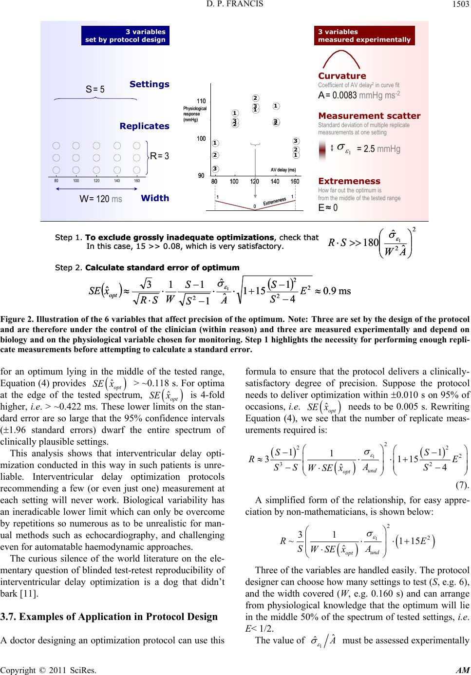

D. P. FRANCIS 1503
80100 120140 160
90
100
110
1
111
12
2
2
2
2
3
3
3
3
3
AV delay (ms)
Physiological
respo nse
(mmHg)
Curvature
Coefficient of AV delay
2
in curve fit
A = 0.0083 mmHg ms
-2
1


Measurement scatter
Extremeness
Standard deviation of multiple replicate
measurements at one setting
How far out the optimum is
from the middle of the tested range
E ≈0
Extremeness
1
1
= 2.5 mm H g
80100 120 140 160
Width
Settings
Replicates
S = 5
W = 120 ms
R = 3
3 variables
set by protocol design3 variables measured experimentally
0
3 variables
set by protocol design


ms9.0
4
1
151
ˆ
ˆ
1
113
ˆ2
2
2
2
1







E
S
S
A
S
S
W
SR
xSE opt


2
2ˆ
ˆ
180 1







 AW SR


Step 1. To exclude grossly inade quate optimizations, che ck that
In this case, 15 >> 0.08, which is very satisfactory.
Step 2. Calculate standard error of optimum
80100 120140 160
90
100
110
1
111
12
2
2
2
2
3
3
3
3
3
AV delay (ms)
Physiological
respo nse
(mmHg)
Coefficient of AV delay
2
in curve fit
A = 0.0083 mmHg ms
-2
Curvature
1


Measurement scatter
Extremeness
Standard deviation of multiple replicate
measurements at one setting
How far out the optimum is
from the middle of the tested range
E ≈0
Extremeness
1
1
= 2.5 mm H g
3 variables
measured experimentally
0
80100 120 140 160
Width
Settings
Replicates
S = 5
W = 120 ms
R = 3
2
2ˆ
ˆ
180 1







 AW SR


Step 1. To exclude grossly inade quate optimizations, che ck that
In this case, 15 >> 0.08, which is very satisfactory.
Step 2. Calculate standard error of optimum

 ms9.0
4
1
151
ˆ
ˆ
1
113
ˆ2
2
2
2
1







E
S
S
A
S
S
W
SR
xSE opt


Figure 2. Illustration of the 6 variables that affect precision of the optimum. Note: Three are set by the design of the protocol
and are therefore under the control of the clinician (within reason) and three are measured experimentally and depend on
biology and on the physiological variable chosen for monitoring. Step 1 highlights the necessity for performing enough repli-
cate measurements before attempting to calculate a standard error.
for an optimum lying in the middle of the tested range,
Equation (4) provides > ~0.118 s. For optima
at the edge of the tested spectrum, is 4-fold
higher, i.e. > ~0.422 ms. These lower limits on the stan-
dard error are so large that the 95% confidence intervals
(1.96 standard errors) dwarf the entire spectrum of
clinically plausible settings.

ˆopt
SE x

ˆopt SE x
This analysis shows that interventricular delay opti-
mization conducted in this way in such patients is unre-
liable. Interventricular delay optimization protocols
recommending a few (or even just one) measurement at
each setting will never work. Biological variability has
an ineradicable lower limit which can only be overcome
by repetitions so numerous as to be unrealistic for man-
ual methods such as echocardiography, and challenging
even for automatable haemodynamic approaches.
The curious silence of the world literature on the ele-
mentary question of blinded test-retest reproducibility of
interventricular delay optimization is a dog that didn’t
bark [11].
3.7. Examples of Application in Protocol Design
A doctor designing an optimization protocol can use this
formula to ensure that the protocol delivers a clinically-
satisfactory degree of precision. Suppose the protocol
needs to deliver optimization within 0.010 s on 95% of
occasions, i.e.


ˆopt SE x needs to be 0.005 s. Rewriting
Equation (4), we see that the number of replicate meas-
urements required is:



1
2
22
2
32
11
1
31
4 ˆund
opt
SS
RE
A SS S
WSEx













15
(7).
A simplified form of the relationship, for easy appre-
ciation by non-mathematicians, is shown below:


1
2
2
31
~1
ˆund
opt
RE
SA
WSEx








15
Three of the variables are handled easily. The protocol
designer can choose how many settings to test (S, e.g. 6),
and the width covered (W, e.g. 0.160 s) and can arrange
from physiological knowledge that the optimum will lie
in the middle 50% of the spectrum of tested settings, i.e.
E< 1/2.
The value of 1
ˆ
ˆ
A

 must be assessed experimentally

D. P. FRANCIS 1504

for each proposed optimization variable. This requires
only a few minutes per subject.
Table 1 shows how this ratio, and other variables, af-
fect the number of replicates needed, R, to achieve the
desired optimization precision.
Although mathematically the tested range W, the re-
quired precision , and the scatter-to-curvature
ratio

ˆopt
SE x
1
The many haemodynamic variables that are affected
by AV delay appear to be initially change proportionally
[12] which suggests that Aund may be approximately the
same proportion of the baseline value of each variable.
The protocol designer desiring small 1
ˆ
ˆ
A

should
therefore favour the variable whose scatter

1
ˆ


is the
smallest proportion of its baseline value.
ˆ
ˆ
A

each have the same impact on the number
of replicates required, in clinical practice

1
ˆ
ˆ4. Limitations
A

has by
far the greatest range of possible values, and the design
process should therefore focus on ensuring that this is
small, if the optimization protocol is to be practical.

Although it is convenient to describe optimization re-
sponses with a parabola, the true underlying shape may
Table 1. Impact of physiology (scatter, curvature and extremeness) and protocol design (number of tested settings, width of
spectrum) on the number of replicates needed for optimization of a desired level of precision.
Distribution of tested settings and physiological characteristics
Number of
replicates per setting
needed to achieve this
Number of
tested
settings
Width of
spectrum
Desired
precision ExtremenessScatter Curvature Scatter/ Curvature ratio
S W


ˆopt SE x E 1
ˆ


ˆ
A
1
ˆ
ˆ
A


R
s s mmHg mmHg·s–2 s
2
6
6
6
6
6
6
6
6
6
6
6
6
6
6
6
6
6
6
6
6
6
6
6
4
6
8
10
12
0.16
0.16
0.16
0.16
0.16
0.16
0.16
0.16
0.16
0.16
0.16
0.16
0.16
0.16
0.16
0.16
0.16
0.16
0.16
0.08
0.12
0.16
0.20
0.16
0.16
0.16
0.16
0.16
0.010
0.005
0.005
0.005
0.005
0.005
0.005
0.005
0.005
0.005
0.005
0.005
0.005
0.005
0.005
0.002
0.005
0.010
0.020
0.005
0.005
0.005
0.005
0.005
0.005
0.005
0.005
0.005
0.5
0.5
0.5
0.5
0.5
0.5
0.5
0.5
0.5
0.5
0
0.25
0.5
0.75
1
0.5
0.5
0.5
0.5
0.5
0.5
0.5
0.5
0.5
0.5
0.5
0.5
0.5
3.9
3
3
3
3
3
1
3
10
30
3
3
3
3
3
3
3
3
3
3
3
3
3
3
3
3
3
3
1194
30
100
300
1000
3000
1000
1000
1000
1000
1000
1000
1000
1000
1000
1000
1000
1000
1000
1000
1000
1000
1000
1000
1000
1000
1000
1000
0.00327
0.1
0.03
0.01
0.003
0.001
0.001
0.003
0.01
0.03
0.003
0.003
0.003
0.003
0.003
0.003
0.003
0.003
0.003
0.003
0.003
0.003
0.003
0.003
0.003
0.003
0.003
0.003
6
21,929
1974
219
20
2
2
20
219
1974
5
9
20
38
64
123
20
5
1
79
35
20
13
24
20
17
14
13
In practice the number of tested settings, width of spectrum, desired precision, and extremeness, all have a limited range of realistic values (as shown). In con-
trast, curvature and scatter have a wide range of possible values and, although rarely formally quantified in research reports, have enormous impact on the
precision of the optimization process. This table can be used for physiological response measures that have any measurement unit (not only mmHg) since it is
the relative size of scatter versus curvature, rather than their absolute values, that is important. For example, if “mmHg” was replaced by “% of value at refer-
ence setting”, the table could without any other alteration be used for any variable such as echo-Doppler velocity-time integral, uncalibrated pressure signal,
bioimpedance-derived stroke volume, or any marker of pulsatility in the peripheral circulation.

D. P. FRANCIS 1505
be more complex. For example, where intrinsic (or even
just fusion) conduction becomes active as AV delay is
lengthened, the data points may deviate upwards from
the parabolic trend, and so fitting to a parabola may bias
the fitted AV delay optimum toward higher values. Nev-
ertheless, the principles in this manuscript would still
hold true. Moreover, in the close vicinity of the optimum,
which is relevant to precise optimization, curvature may
be closer to parabolic.
Merely applying formulae will not make optima more
precise. Only selecting a physiological variable of suita-
bly low 1
ˆ
ˆ
A

ratio, and taking time to conduct
enough measurements (shown in Equation (7)), can im-
prove precision. Lack of interest in scatter and curvature
in a doctor conducting optimization is as uninspiring as
lack of interest in wings and engines in an aircraft pilot.

5. Conclusions
The practical implications may be summarized from in-
spection of each factor in Equation (6) in turn. To obtain
precise clinical optima:
 most importantly, either commit enough resources to
obtain enough measurements, or do not embark on
optimization;
 cover a wide range of pacemaker settings while re-
maining within the parabolic region of the response
curve;
 choose a physiological variable with as narrow a
random variability (in relation to its sensitivity to
pacemaker setting change) as possible; and
 if possible, design the spectrum of settings tested so
that the true optimum will lie near its middle rather
than at an extreme.
Clinicians treating patients and scientists designing
and conducting studies have not had simple, quick me-
thods to establish the uncertainty in planned or actual
optimization procedures. As a result, patients may be
undergoing apparent optimization procedures that are in
fact worsening the programming of their pacemaker.
Moreover without methods for recognizing unreliable
optimizations, clinicians finding the optimum appearing
to change every 1 or 2 years may feel compelled to carry
out worthless optimization procedures more frequently,
[8] which wastes clinical resources and may be harmful
to patients.
The results in this paper permit easy quantification of
uncertainty of the optimum of a cardiac resynchroniza-
tion therapy pacemaker. They help patients gain the best
physiological benefit, help doctors design protocols that
deliver efficient and reliable optimization, and assist in
distinguishing genuine change in patient physiology over
time, versus random noise.
An unexamined optimization is not worth doing.
6. Acknowledgements
The author is supported by a Senior Research Fellowship
(FS/10/038) from the British Heart Foundation.
7. References
[1] W. T. Abraham, W. G. Fisher and A. L. Smith, “Cardiac
Resynchronization in Chronic Heart Failure,” New Eng-
land Journal of Medicine, Vol. 346, 2002, pp. 1845-1853.
doi:10.1056/NEJMoa013168
[2] A. Kyriacou, P. A. Pabari, and D. P. Francis, “Cardiac
Resynchronization Therapy Is Certainly Cardiac Therapy,
But How Much Resynchronization and How Much
Atrioventricular Delay Optimization?” Heart Failure Re-
views, 2011, Article in Press.
doi:10.1007/s10741-011-9271-1
[3] J. G. Cleland, J. C. Daubert, E. Erdmann, N. Freemantle,
D. Gras, L. Kappenberger and L. Tavazzi, “Cardiac Re-
synchronization-Heart Failure (CARE-HF) Study Inves-
tigators. The Effect of Cardiac Resynchronization on
Morbidity and Mortality in Heart Failure,” New England
Journal of Medicine, Vol. 352, No. 15, 2005, pp. 1539-
1549. doi:10.1056/NEJMoa050496
[4] A. Auricchio, C. Stellbrink, S. Sack, M. Block, J. Vogt, P.
Bakker, C. Huth, F. Schöndube, U. Wolfhard, D. Böcker,
O. Krahnefeld and H. Kirkels, “Pacing Therapies In
Congestive Heart Failure (PATH-CHF) Study Group.
Long-Term Clinical Effect of Hemodynamically Opti-
mized Cardiac Resynchronization Therapy in Patients
With Heart Failure and Ven-Tricular Conduction Delay,”
Journal of the American College of Cardiology, Vol. 39,
No. 12, 2002, pp. 2026-2033.
doi:10.1016/S0735-1097(02)01895-8
[5] M. D. Bogaard, P. A. Doevendans, G. E. Leenders, P.
Loh, R. N. Hauer, H. van Wessel and M. Meine, “Can
Optimization of Pacing Settings Compensate for a Non-
Optimal Left Ventricular Pacing Site?” Europace, Vol.
12, No. 9, 2010, pp. 1262-1269.
doi:10.1093/europace/euq167
[6] I. E. van Geldorp, T. Delhaas, B. Hermans, K. Vernooy,
B. Broers, J. Klimusina, F. Regoli, F. F. Faletra, T. Moc-
cetti, B. Gerritse, R. Cornelussen, J. Settels, H. J. Crijns,
A. Auricchio and F. W. Prinzen, “Comparison of a Non-
Invasive Arterial Pulse Contour Technique and Echo
Doppler Aorta Velocity-Time Integral on Stroke Volume
Changes in Optimization of Cardiac Resynchronization
Therapy,” Europace, Vol. 13, No. 1, 2011, pp. 87-95.
doi:10.1093/europace/euq348
[7] Z. I. Whinnett, J. E. Davies, G. Nott, K. Willson, C. H.
Manisty, N. S. Peters, P. Kanagaratnam, D. W. Davies, A.
D. Hughes, J. Mayet and D. P. Francis, “Efficiency, Re-
producibility and Agreement of Five Different Hemo-
dynamic Measures for Optimization of Cardiac Resyn-
chronization Therapy,” International Journal of Cardio-
logy, Vol. 129, No. 2, 2008, pp. 216-226.

D. P. FRANCIS 1506
doi:10.1016/j.ijcard.2007.08.004
[8] P. A. Pabari, K. Willson, B. Stegemann, I. E. van Geldorp,
A. Kyriacou, M. Moraldo, J. Mayet, A. D. Hughes and D.
P. Francis, “When Is an Optimization Not an Optimiza-
tion? Evaluation of Clinical Impli-Cations of Information
Content (Signal-to-Noise Ratio) in Optimization of Car-
diac Resynchronization Therapy, and How to Measure
and Maximize It,” Heart Failure Reviews, Vol. 16, No. 3,
2011, pp. 277-290. doi:10.1007/s10741-010-9203-5
[9] W. T. Abraham, D. Gras, C. M. Yu, L. Guzzo and M. S.
Gupta, “Rationale and Design of A Randomized Clinical
Trial to Assess the Safety and Efficacy of Frequent Opti-
mization of Cardiac Resynchronization Therapy: The
Frequent Optimization Study Using the Quickopt Method
(FREEDOM) Trial,” American Heart Journal, Vol. 159,
No. 6, 2010, pp. 944-948. doi:10.1016/j.ahj.2010.02.034
[10] Z. I. Whinnett, J. E. R. Davies, K. Willson, C. H. Manisty,
A. C. Chow, R. A. Foale, D. W. Davies, A. D. Hughes, J.
Mayet and D. P. Francis, “Haemodynamic Effects of
Changes in AV and VV Delay in Cardiac Resynchroniza-
tion Therapy Show a Consistent Pattern: Analysis of
Shape, Magnitude and Relative Importance of AV and
VV Delay,” Heart, Vol. 92, 2006, pp. 1628-1634.
doi:10.1136/hrt.2005.080721
[11] A. C. Doyle, “The Curious Incident of the Dog in the
Night-Time,” Strand Magazine, Vol. 4, No. 4, 1892, pp.
645-660.
http://www.archive.org/download/StrandMagazine24/
Strand24_text.pdf
[12] C. H. Manisty, A. Al-Hussaini, B. Unsworth, R. Baruah,
P. A. Pabari, J. Mayet, A. D. Hughes, Z. I. Whinnett and
D. P. Francis, “The Acute Effects of Changes to AV De-
lay on Blood Pressure and Stroke Volume: Potential Im-
plications for Design of Pacemaker Optimization Proto-
cols,” Circulation: Arrhythmia and Electrophysiology,
Article in Press.
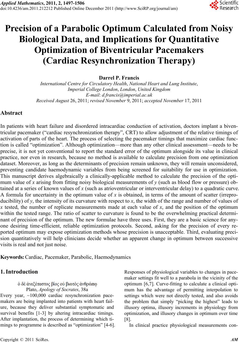