Journal of Modern Physics
Vol.3 No.8(2012), Article ID:21688,9 pages DOI:10.4236/jmp.2012.38102
On the Quantization of One-Dimensional Conservative Systems with Variable Mass
Departamento de Física de la Universidad de Guadalajara, esq. Calzada Olmpica, Guadalajara, México
Email: gulopez@udgserv.cencar.udg.mx
Received May 30, 2012; revised June 25, 2012; accepted July 18, 2012
Keywords: Mass Variation; Quantization; Constant of Motion; Hamiltonian
ABSTRACT
The Hamiltonian associated to the mass variable system is constructed from first principles through finding a constant of motion of the system. A comparison is made of the classical motion of a body with its mass position depending in the (x,v) space and (x,p) space which are defined by the constant of motion and the Hamiltonian, for a particular model of mass variation. As one could expected, these motion looks different on these spaces. The quantization of the harmonic oscillator with this mass variation is done, and a comparison is made by using the usual Hamiltonian approach with the proposed quantization of the constant of motion approach. This comparison is done at first order in perturbation theory, and one sees a difference between both approaches which can, in principle, be measured.
1. Introduction
Mass variation problems for classical mechanics has a long history [1] and important applications have been studied on the dynamics of the Universe as black hole formation [2,3], where they have been known as GyldenMeshcherskii problems [4-11]. These types of problems are not free from controversy in the way they must be formulated and their relation with Galileo’s transformation [12]. In addition, these systems are becoming more and more important in quantum mechanics systems since the discovery of the neutrinos mass oscillations problem [13] and [14], the kinetic theory of dusty plasma [15], propagation of electromagnetic waves in a dispersivenonlinear media [16], and other possible applications in fluid dynamics [17].
The approach used so far to study these systems follows guessed Lagrangian or Hamiltonian with include the mass variation of the system [18-20]. Above all, there is not right mathematical justification for this approach. Therefore, one may considered that to find the Hamiltonian for a mass variation system, one must do it from first principles, Newtonian’s mechanics, and this can be done by using a well known approach for one dimensional autonomous system to construct the associated Lagrangian and Hamiltonian of the system [21-23]. Once these expressions are gotten, one can proceed to make the quantization of the system [24]. On the other hand, there has been a proposed extension for the non relativistic quantum mechanics for autonomous systems based on the use of the constant of motion instead of the Hamiltonian in the Schrödinger equation [25]. Therefore, in this paper the Hamiltonian and the constant of motion are found for several conservative systems with position depending mass, using a model for the mass variation. The trajectories of the motion on the (x,v) and (x,p) spaces are shown to see the difference of this description. The quantization of the mass position depending systems is analyzed using the constant of motion and the Hamiltonian approaches, and finally, the spectrum of the harmonic oscillator are calculate at first order perturbation theory.
2. Constant of Motion and Hamiltonian
Consider a one-dimensional motion of a body with mass position depending,  , and which is affected by a conservative force
 . This system is governed by Newton’s equation of motion [1]
 (1)
(1)
where v represents the velocity of the body. Since one has the expression
 (2)
(2)
where one has defined , the equation of motion can be written as the following system
 (3)
(3)
which in turns, this equation can be written as the following autonomous dynamical system
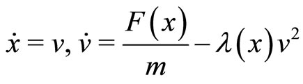 (4)
(4)
where  has defined as
 (5)
(5)
This autonomous system is dissipative for  and anti dissipative for
  because of the quadratic term in the velocity. A constant of motion of this system is a function
  which satisfies the first order partial differential equation
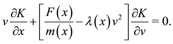 (6)
(6)
The general solution of this equation is given by , where G is an arbitrary function, and C is the characteristic curve given by
 (7)
(7)
Suppose  of the form
 , where one demands that
 . In addition, assuming that
 , one gets the usual constant of motion of the conservative system with constant mass (so called “Energy of the System”). Then, one can select the functionality of G of the form
 (8)
(8)
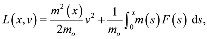
such that under the mentioned conditions for g, one gets the energy of the system as a particular limit. The resulting constant of motion of the system is
 (9)
(9)
Given the constant of motion of a one-dimensional autonomous system, the Lagrangian for this system is determine through the well known expression ([21-23])
 (10)
(10)
Using this expression with Equation (9), it follows that
 (11)
(11)
The generalized linear momentum,  , is given by
 (12)
(12)
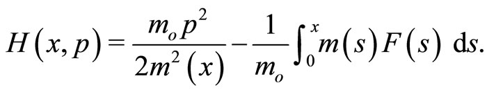
and the Hamiltonian of the system,  , is deduced as
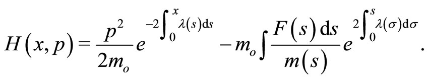 (13)
(13)
Since from Equation (5) one has that
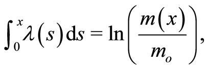 (14)
(14)
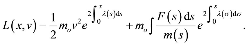
The constant of motion, Lagrangian, generalized linear momentum, and Hamiltonian are written as
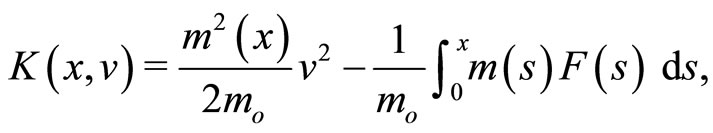 (15)
(15)
 (16)
(16)
 (17)
(17)
and
 (18)
(18)
Defining the effective potential as
 (19)
(19)
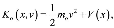
the constant of motion and Hamiltonian have the following form
 (20)
(20)
and
 (21)
(21)
To be able to continue with analysis, one needs a model for the variation of mass, . Let us assume that
  is given by
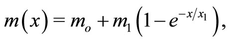 (22)
(22)
where  and
and  and
and  determines the asymptotic distance where the mass would be
 . One will have and increasing of mass going from
  to
to  if
if , and vise versa if
 . For this model, The effective potential is given by
 (23)
(23)
where  is the usual conservative potential due to the force
 ,
,
 (24)
(24)
The trajectories in the space  are determined by the constant of motion Equation (20), given the initial conditions
  and
and  The trajectories in the space
  are determined by Equation (21) with the initial conditions
  and
and , where Equation (17) relates both initial conditions. Figures 1 and 2 show the trajectories in the space
  and
and  for a constant force
 . Figures 3 and 4 show the trajectories in the spaces
  and
and  for a Coulomb Force
  (zero potential is taken at
  ). Figures 5 and 6 show the trajectories in the spaces
  and
and  for the Hook’s law (harmonic oscillator)
  (for the dissipative case
 ). Gross continuous black line represents
 , dotted lines correspond to
  and continuous lines to
  The following values have been used to make this plots (units MKS),

 and
and  (in their respective units).

Figure 1. Constant of motion trajectories, F = f.

Figure 2. Hamiltonian trajectories, F = f.
As one can see from these plots, the effect of the first terms in Equations (20) and (21) is clearly marked on these trajectories. The constant of motion brings about some “regular” behavior meanwhile the Hamiltonian brings about some type of little odd behavior due to expression (17).
From Equations (23), (20) and (21) one sees that the constant of motion and the Hamiltonian can be written as
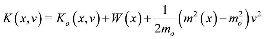 (25)
(25)
and
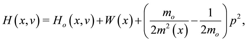 (26)
(26)
where the terms ,
,  and
and  are given by
 (27)
(27)
 (28)
(28)
and
 (29)
(29)
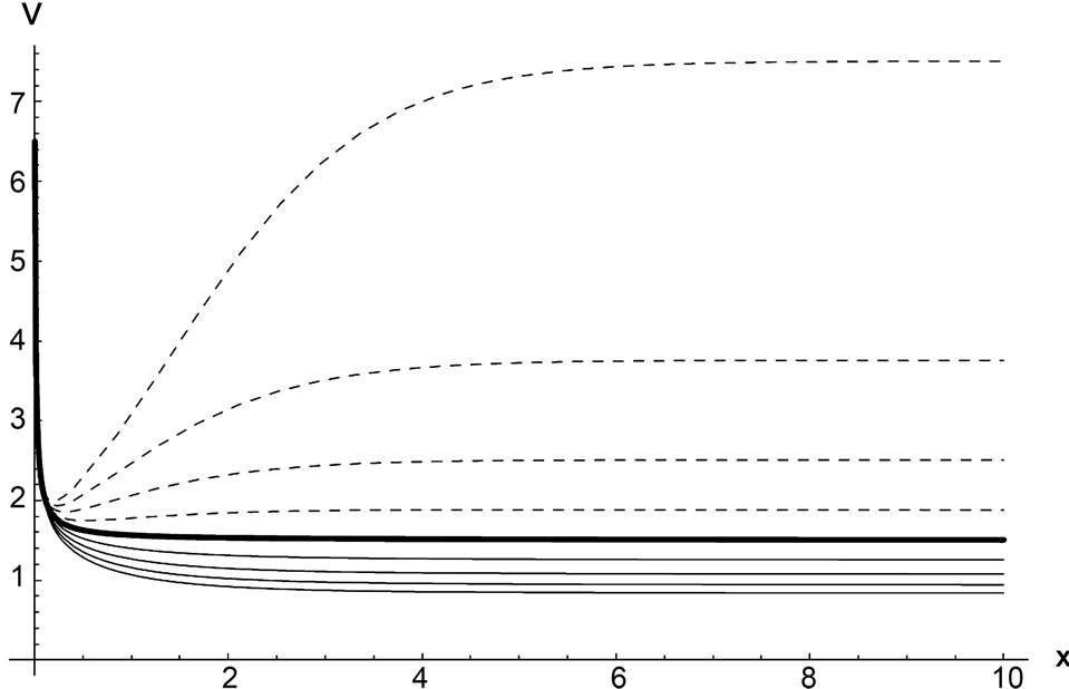
Figure 3. Constant of motion trajectories, F = –k'/x2.
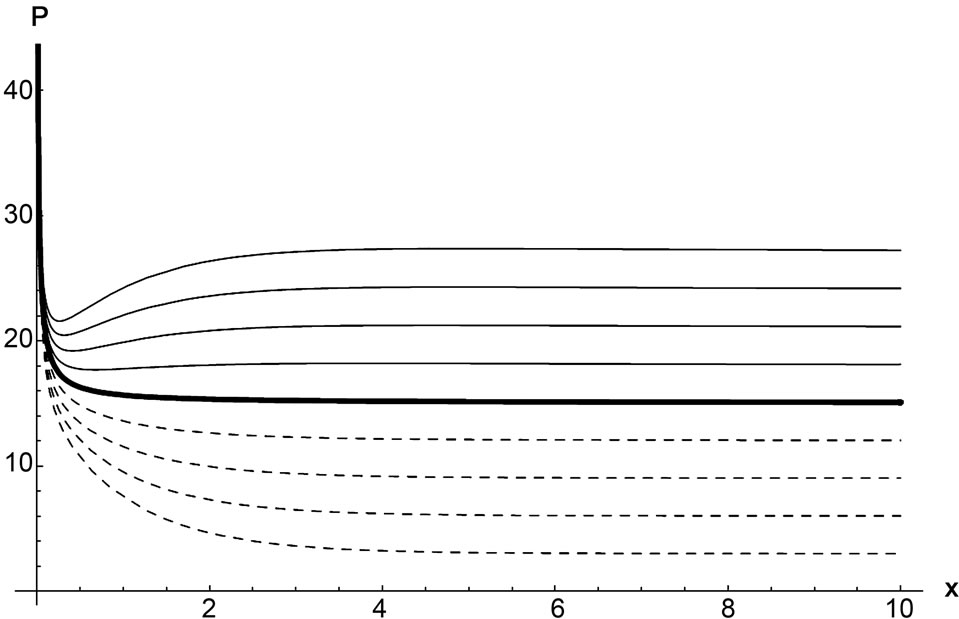
Figure 4. Hamiltonian trajectories, F = –k'/x2.

Figure 5. Constant of motion trajectories, F = –kx.

Figure 6. Hamiltonian trajectories, F = –kx.
This form of writing the constant of motion and the Hamiltonian is suitable for quantization studies. Before leaving this classical part, it is necessary to make some observations about the motion of the body and its mass position dependence. First, in our mass position dependence model, Equation (22), it has been assumed that the asymptotic ( ) mass value is given by
 . If the body oscillates (harmonic oscillator), in addition to damping-antidamping effect due to the term with
  in Equation (3), one must consider the effect of decreasing (for
 ) and increasing (for
 ) of mass effect during these oscillations. Second, if one would like to consider pure decreasing of mass during these oscillations, it is necessary to change the model for
 . Third, if one wants to consider pure damping effect during these oscillations, this will only happen if
  for
for  and
and  for
for , [26]. Finally, if
  (our model) or
  for any position “x”, the damping-antidamping effect will appear.
3. Quantization with Mass Position Depending Systems
The usual Schrödinger quantization approach is based on the association of an Hermitian operator to the Hamilton function, [27,28], and the solution of a linear complex partial differential equation for the wave function,  ,
,
 (30)
(30)
where  is the Hermitian operator associated to the generalized linear momentum,
  ,
,  is the Plank constant divided by
 , having the confutation relation
  (with “I” the identity operator) in the basis
  of the Weyl algebra. However, as a possible extension of this quantization approach, there is the proposal of using the constant of motion, instead of the Hamiltonian, in the Schrödinger equation, where an Hermitian operator is associated to the constant of motion function, and the Schrödinger like equation is solved for the wave function,
 (31)
(31)
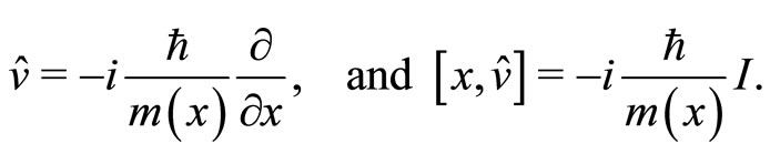
where  is the Hermitian operator associated to the velocity,
  , satisfying the obvious commutation relation
 (32)
(32)
These realtions can be assumed to be valid for position mass depending as
 (33)
(33)
Of course, for constant mass conservative systems, there is not difference at all between both approaches since the relation between the generalized linear momentum and the velocity of the body is really trivial, . However, as we have seen previously, for mass position depending systems this relation is not trivial any more, Equation (17). Therefore, to find out the possibility for the quantization of the constant of motion to make physical sense, it is necessary to look for a system where both approaches differs, and to see experimentally whether or not it makes sense. Mass position depending systems have indeed this property because of the Equation (17).
For autonomous systems, one does not need, of course, to fully solve the Equations (30) and (31) to see whether or not there is a difference on both approaches. To see this, it is enough to look at their spectra, and this spectra can even be calculated at first order in perturbation theory. Even more, one can see these spectra just a second order in the Taylor expansion of the mass position depending. Doing this with the Equations (25)-(27), one gets
 (34)
(34)
and
 (35)
(35)
where the function  is defined as
 (36)
(36)
To associate a Hermitian operator to these functions, one knows that there is an ambiguity, not resolved yet by any experiment, on selecting a proper Hermitian operator to make the quantization. Although one could normally follow Weyl approach [29] and [30], it is easier to take the following approach by noticing the following for polynomials operators: given the Hermitian operators  and
and  to the functions A and B, the operator
  is an Hermitian operator for any integer number “n”. In this way, the following Hermitian operators can be associated to the product of functions
 (37)
(37)
 (38)
(38)
and
 (39)
(39)
Taking the following identifications  and
and  or
or , it follows that the Hermitian operators associated to the expressions (34) and (36) are given by
 (40)
(40)
and
 (41)
(41)
Using the commutation relations  and
and
 (42)
(42)
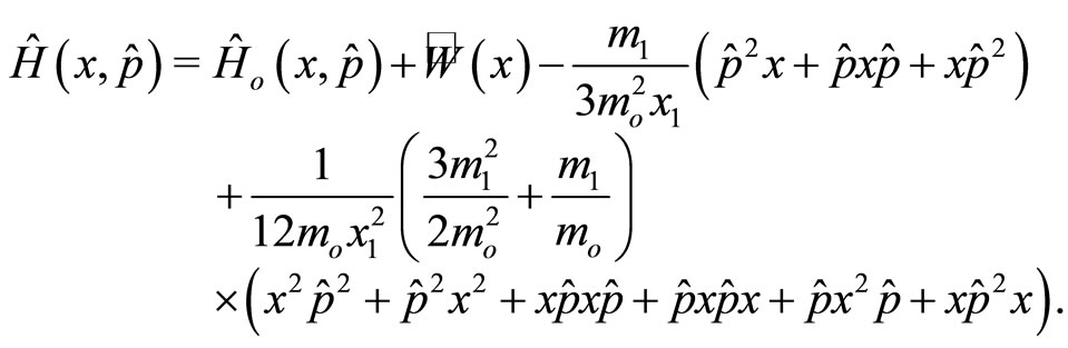
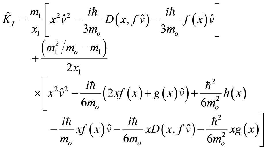
one gets the following expressions for the constant of motion and Hamiltonian operators
 (43)
(43)
and
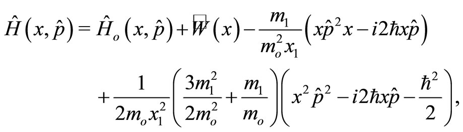 (44)
(44)
where the functions  and
and , and the operator
  have been defined as
 (45)
(45)
 (46)
(46)
 (47)
(47)
Now, since Equations (30) and (31) represent autonomous systems, the solution of these equation are reduced to the solution of eigenvalue problems
 (48)
(48)
and
 (49)
(49)
Considering on Equations (43) and (44) that the terms appearing on the right hand side are small with respect the terms  and
and , the modification of the
  and
and  spectra can be calculated just at first order in perturbation theory to see whether or not there is a significant difference in their predictions. In this case, one must have that the eigenfunctions and eigenvalues are the same for both approaches when
 ,
,
 (50)
(50)
Then, at first order perturbation theory, the eigenvalues would be given by
 (51)
(51)
and
 (52)
(52)
where  is the expectation value of the function
  in the state
 , and
, and  and
and  represent the remaining terms of the Equations (43) and (44),
 (53)
(53)
and
 (54)
(54)
4. Harmonic Oscillator with Variable Mass
The harmonic oscillator with  in the Weyl algebra basis
  [31] has the following characteristics
 (55)
(55)
with the following identifications
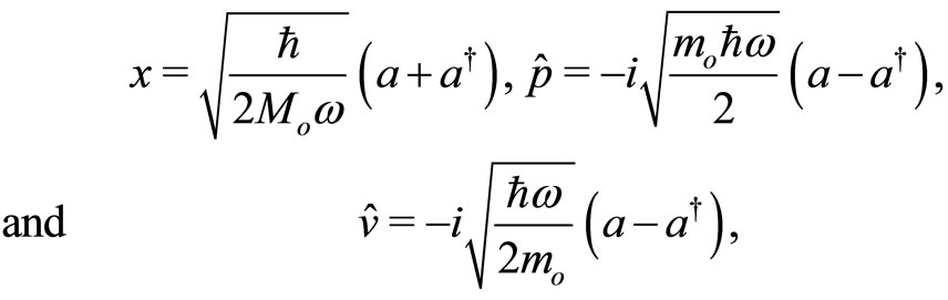 (56)
(56)
and having the well known properties
 (57)
(57)
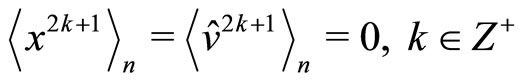
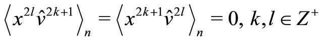
Note that all the expectation values of monomial terms of odd power have zero values. The expression for  up to fourth order in “x” is given by
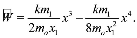 (58)
(58)
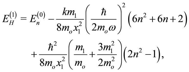
Thus, using the expectation values given in the appendix, the expectation value of the terms appearing in Equations (53) and (54) can be calculated, resulting the following eigenvalues at first order
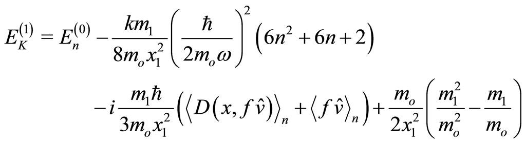 (59)
(59)
and
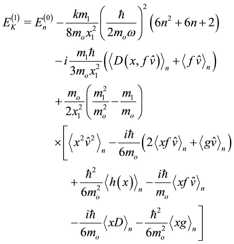 (60)
(60)
where one has used the definition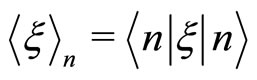 . Let us define the following parameter J as
 (61)
(61)
This parameter represents the relative variation of the eigenvalues of the constant of motion quantization and the Hamiltonian quantization approaches. Figure 7 shows this parameter as a function of  (relative change of mass), considering that
 and
and  (ground state), for
  with
with  (dotted line), 2, 4, 6, and 8 (progressively). Figure 8 shows J as a function of
  considering the same previous values for the parameters but for j = 1 and
  with
with  (dotted line), 20, 40, 60 and 80. Figure 9 shows again J vs
  with the same values for the parameters as before but with
  and for
  (dotted line), 2, 4, 6, and 8. As one can see from these plots, even for a relatively small change in the mass of the body, the difference of

Figure 7. J vs m1/mo for various “x1”.

Figure 8. J vs m1/mo for various “mo”.

Figure 9. J vs m1/mo for various “n”.
the eigenvalues for both approaches (J) could be relatively large. Thus, this suggest the it can be observable experimentally, opening up the possibility to see whether or not the quantization of constant of motion makes sense for mass variable quantum systems.
5. Conclusion
A mathematical consistent approach has been used to deduce the constant of motion, Lagrangian, and Hamiltonian for a mass position depending non relativistic classical systems. The trajectories on the spaces ( ) and (
 ) were given for constant force, Coulomb type force, and Hook force with a chosen model for the mass variation. The dependence of the generalized linear momentum with respect the position and the velocity of the body makes the plots in the space (
 to look quite different from those in the space (
 ). In addition, an study was made about the quantization of the constant of motion, as an extension approach of the usual Hamiltonian quantization approach The harmonic oscillator with mass position depending was used for this study. One observed that, already, at first order perturbation theory, a significant difference on the spectra of the constant of motion and Hamiltonian approaches can be significant, bringing about the possibility for this difference to to be observed experimentally.
REFERENCES
- H. Goldstein, “Classical Mechanics,” Addison-Wesley, Boston, 1950.
- F. W. Helhl, C. Kiefer and R. J. K. Metzler, “Black Holes: Theory and Observation,” Springer-Verlag, Berlin, 1998.
- P. W. Daly, “The use of Kepler trajectories to calculate Ion Fluxes at Multi-Gigameter Distances from Comet Halley,” Astronomy and Astrophysics, Vol. 226, no. 1, 1989, pp. 318-334.
- H. Gylden, “Die Bahnbewegungen in Einem Systeme von zwei Körpern in dem Falle, dass die Massen Veränderungen Unterworfen Sind,” Astronomy and Astrophysics, Vol. 109, no. 1-2, 1884, pp. 1-6. doi:10.1002/asna.18841090102
- I. V. Meshcherskii, “Ein Specialfall des Gyldn’schen Problems,” Astronomische Nachrichten, Vol. 132, no. 3153, 1893, p. 93.
- I. V. Meshcherskii, “Ueber die Integration der Bewegungsgleichungen im Problemezweier Krper von Vernderlicher Masse,” Astronomische Nachrichten, Vol. 159, no. 15, 1902, pp. 229-242.
- E. O. Lovett, “Note on Gyldén’s equations of the problem of two bodies with Masses Varying with the time,” Astronomische Nachrichten, Vol. 158, no. 2, 1902, pp. 337-344. doi:10.1002/asna.19021582202
- J. H. Jeans, “The effect of varying mass on a binary system,” Monthly Notices of the Royal Astronomical Society, Vol. 85, 1925, p. 912.
- L. M. Berkovich, “Gylden-Meščerskii problem,” Celestial Mechanics and Dynamical Astronomy, Vol. 24, No. 4, 1981, pp. 407-429. doi:10.1007/BF01230399
- A. A. Bekov, “Integrable cases and motion trajectories in the Gylden-Meshcherskii problem,” Soviet Astronomy, Vol. 33, 1989, pp. 71-78.
- C. Prieto and J. A. Docobo, “Analythic solution of the Two-Body Problem with Slowly Decreasing Mass,” Astronomy and Astrophysics, Vol. 318, 1997, pp. 657-661.
- G. V. López, “About Galilean transformation on a mass Variable System and Two Bodies Gravitational System with Variable Mass and Dampen-Anti Damping Effect Due to Star Wind,” 2012. http://arxiv.org/abs/1203.0495v1
- H. A. Bethe, “Possible Explanation of the Solar-Neutrino Puzzle,” Physical Review Letters, Vol. 56, No. 12, 1986, pp. 1305-1308. doi:10.1103/PhysRevLett.56.1305
- E. D. Commins and P. H. Bucksbaum, “Weak Interactions of Leptons and Quarks,” Cambridge University Press, Cambridge, 1983.
- A. G. Zagorodny, P. P. J. M. Schram and S. A. Trigger, “Stationary Velocity and Charge Distributions of Grains in Dusty Plasmas,” Physical Review Letters, Vol. 84, No. 16, 2000, pp. 3594-3597. doi:10.1103/PhysRevLett.84.3594
- O. T. Serimaa, J. Javanainen and S. Varró, “Gauge-independent Wigner Functions: General formulation,” Physical Review A, Vol. 33, No. 5, 1986, pp. 2913-2927. doi:10.1103/PhysRevA.33.2913
- I. Ye. Terapov, “On Some Fundamental Problems of the Variable-Mass Continuum Mechanics,” International Journal of Fluid Mechanics Research, Vol. 28, No. 4, 2001, pp. 152-174.
- C. Quesne, B. Bagchi, A. Banerjee and V. M. Tkachuk, Hamiltonians with Position-Dependent Mass, Deformations and Supersymmetry,” Bulgarian Journal of Physics, Vol. 33, 2006, pp. 308-318.
- Y. Hamdouni, “Motion of Position-Dependent Effective Mass as a Damping-Antidamping Process: Application to the Fermi gas and the Morse potential,” Journal of Physics A: Mathematical and Theoretical, Vol. 44, No. 38, 2011, Article ID: 385301. doi:10.1088/1751-8113/44/38/385301
- M. Çapak, Y. Cançelik and Ö. L. Ünsal, S. Tay and B. Gönül, “An extended scenario for the Schrödinger equation,” Journal of Mathematical Physics, Vol. 52, No. 10, 2011, Article ID: 102102. doi:10.1063/1.3646371
- J. A. Kobussen, “Some comments on the lagrangian formalism for systems with general velocity dependent forces,” Acta Physica Austriaca, Vol. 51, 1979, pp. 293- 309.
- C. Leubner, “Inequivalent lagrangians from constants of the motion,” Physical Review A, Vol. 86, No. 2, 1981, pp. 68-70. doi:10.1016/0375-9601(81)90166-3
- G. López, “One-Dimensional Autonomous Systems and Dissipative Systems,” Annals of Physics, Vol. 251, no. 2, 1996, pp. 372-383. doi:10.1006/aphy.1996.0118
- G. Lópezand and G. González, “Quantum Bouncer with Dissipation,” International Journal of Theoretical Physics, Vol. 43, No. 10, 2004, pp. 1999-2008. doi:10.1023/B:IJTP.0000049005.73750.c0
- G. López and P. López, “Velocity Quantization Approach of the One-Dimensional Dissipative Harmonic Oscillator,” International Journal of Theoretical Physics, Vol. 45, No. 4, 2006, pp. 753-742. doi:10.1007/s10773-006-9064-9
- G. López, “Restricted Constant of Motionfor the OneDimensional Harmonic Oscillator with Quadratic Dissipation and Some Consequences in Statistic and Quantum Mechanics,” International Journal of Theoretical Physics, Vol. 79, No. 4, 2001, pp. 71-79. doi:10.1023/A:1011972700121
- A. Messiah, “Quantum Mechanics vol. I,” John Wiley and Sons, New York, 1958.
- P. A. M. Dirac, “The Principles of Quantum Mechanics,” 4th edition, Oxford Science Publications, Oxford, 1992.
- H. Weyl, “Quantenmechanik und Gruppentheorie,” Zeitschrift für Physick, Vol. 46, No. 1-2, 1927, pp. 1-46. doi:10.1007/BF02055756
- R. Kubo, “Wigner Representation of Quantum Operators and its Applications to Electrons in a Magnetic Field,” Journal of the Physical Society of Japan, Vol. 19, 1964, pp. 2127-2139. doi:10.1143/JPSJ.19.2127
- C. Cohen-Tannoudji, B. Diu and F. Laloë, “Quantum Mechanics vol. I,” John Wiley and Sons, New York, 1977.
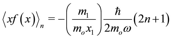
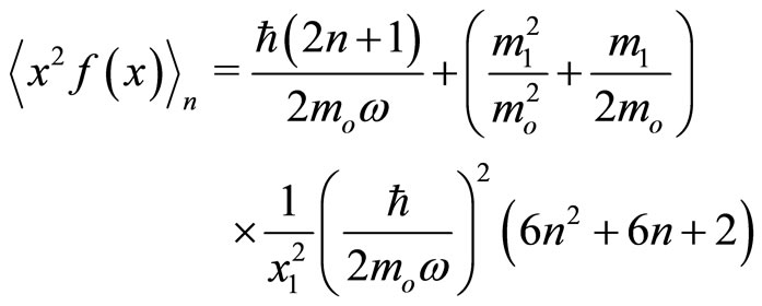
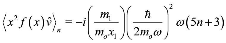
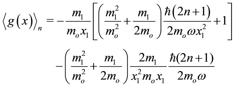
Appendix
List of expectation values.
 (A1)
(A1)
 (A2)
(A2)
 (A3)
(A3)
 (A4)
(A4)
 (A5)
(A5)
 (A6)
(A6)
 (A7)
(A7)
 (B1)
(B1)
 (B2)
(B2)
 (B3)
(B3)
 (B4)
(B4)
 (B5)
(B5)
 (B6)
(B6)
 (B7)
(B7)
 (C1)
(C1)
 (C2)
(C2)
 (C3)
(C3)
 (C4)
(C4)
 (D1)
(D1)
 (D2)
(D2)
 (D3)
(D3)
 (E1)
(E1)
 (E2)
(E2)
 (E3)
(E3)