Applied Mathematics
Vol.4 No.8A(2013), Article ID:35185,8 pages DOI:10.4236/am.2013.48A016
The Catastrophe Map of a Two Period Production Model with Uncertainty
1Department of Statistics, University College London, London, UK
2Department of Mathematics, University of Sussex, East Sussex, UK
Email: p.stiefenhofer@ucl.ac.uk
Copyright © 2013 Pascal Stiefenhofer. This is an open access article distributed under the Creative Commons Attribution License, which permits unrestricted use, distribution, and reproduction in any medium, provided the original work is properly cited.
Received June 5, 2013; revised July 5, 2013; accepted July 12, 2013
Keywords: Differential Topologyl; General Equilibrium; Uncertainty; Production
ABSTRACT
This paper shows existence and efficiency of equilibria of a two period production model with uncertainty as a consequence of the catastrophe map being smooth and proper. Its inverse mapping defines a finite covering implying finiteness of equilibria. Beyond the extraction of local equilibrium information of the model, the catastrophe map renders itself well for a global study of the equilibrium set. It is shown that the equilibrium set has the structure of a smooth submanifold of the Euclidean space which is diffeomorphic to the sphere implying connectedness, simple connectedness, and contractibility.
1. Introduction
This paper considers a two period production model with uncertainty. The time structure and associated uncertainty is described by a finite number of uncertain states of the world. It is assumed that all firms are owned by the consumers according to an exogenously determined ownership structure. This economic scenario describes the private ownership model discussed in Debreu [1] where the objective of each firm is to maximize profits. The seminal paper of this model without uncertainty dates back to the path breaking paper by Arrow and Debreu [2].
In this paper, we show that many economically interesting equilibrium properties of the two period production model with uncertainty can be derived from the catastrophe map. For that purpose we follow the mathematical approach discussed in Balasko [3] and in Dierker [4].
More specifically, we describe the set of solutions of all two period production economies and explore its structure. It is shown that this set is a smooth submanifold of the Euclidean space which is diffeomorphic to the sphere. A study of some of the properties of the catastrophe map enables us to characterize the set of economies into sets with various properties, such as economies with singular equilibria, economies with multiple equilibria, and economies with catastrophes, where equilibrium behavior is more difficult to study. Most of these properties have been studied in the context of exchange economies [5] or simple production economies [6-10] or Balasko (Preprint 2011) for example1. This paper generalizes the economic scenario by adding more structure to the model of the firm and thus moving towards a more realistic model where time and uncertainty is present.
The structure of the paper is as follows: Section 1 is an introduction. Section 2 introduces the economic scenario and states a definition of economic equilibrium. Section 3 explores the topological structure of the equilibrium set of all two period production economies with uncertainty. The next section states equilibrium properties of the model such as existence, efficiency and finiteness of equilibria. The final section is a conclusion.
2. The Long Run Private Ownership Production Model with Uncertainty
We describe the two period private ownership production model  introduced in Debreu ([1], chapter 7). Uncertainty is defined by a finite set of mutually exclusive and exhaustive states of nature denoted by
 , where
  is the certain event in time period one and
  are the uncertain events in time period two. In total there are
  states of nature. There are
  consumers,
  producers, and
  physical goods. For all consumers
 , a consumption bundle is a collection of vectors
![]() where consumption in a particular state
where consumption in a particular state  is a vector
 . Associated with physical commodities is a set of normalized pricesdenoted
 .
.
Consumers are further endowed with a fraction  of the profits of each firm.
  represents the exogenously determined ownership structure of the private ownership production economy. It satisfies for each
  and
and , 0 ≤ θij ≤ 1, and
 . Denote the set of ownership structures
 .
.
Consumers are endowed with a collection of vectors of initial resources denoted by
![]() , where initial endowments in a particular state
, where initial endowments in a particular state  is a vector
 . Consumer
 is further characterized by a smooth Marschallian demand function
 , where
 is defined for price vector
  and wealth level
 , [11], where
  for all
 .
.
Producers are characterized by production sets and their smooth supply functions. The main property of the long run production model is that all activities of the firm are variable. An activity  is a collection of vectors
![]() , where an activity in state
, where an activity in state  is a vector of inputs
 , and
, and
 is the associated vector of outputs in state
 . Let
. Let  denote the smooth supply function of firm
 , where
  is defined on the set of normalized prices. Standard assumptions of smooth production economies introduced in [1] hold for each production set
 . In particular
  is convex,
  , and
, and  has a strictly positive Gaussian curvature for every
 . These assumptions imply that supply functions are smooth.
Equilibrium 
Each consumer  chooses a utility maximizing consumption bundle
  at fixed
  and
and  satisfying his budget constraints. Each producer
  chooses profit maximizing net activities
  at competitive prices
 . Let
. Let
 (1)
(1)
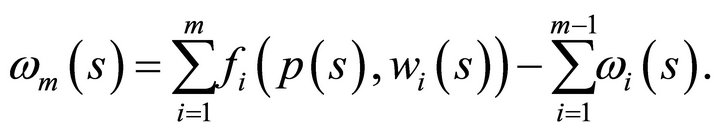
be the market excess demand function in state  . Then, market clearance requires demand to equal supply in each market and uncertain state of the world. Hence
An equilibrium is a price vector  which satisfies this equation for a fixed distribution of initial resources and exogenously given ownership structure. An equilibrium pair is an equilibrium price vector
  with associated
 . An equilibrium allocation is an allocation
  associated with an equilibrium price
 . The model of the consumer is to solve a constraint optimization problem. This requires a consumer to maximize utility subject to a sequence of
  budget constraints. Hence, each consumer

where  is the consumer’s smooth2 utility function. The production adjusted consumer budget set is defined by
The model of the producer is to maximize profits. Each producer solves a constraint optimization profit maximization problem. Hence, each 

where the state dependent production set  for all
  satisfies the assumptions of Debreu [1].
Definition 1. An equilibrium of the two period private ownership production model with uncertainty  is a price vector
  at fixed pair
  if for utility maximizing consumers
  and profit maximizing producers
 (2)
(2)
An equilibrium allocation is a pair  associated with an equilibrium price vector
  for fixed parameters
 . Let denote the mathematical operation defined by a state by state inner product. There are
  equilibrium equations less
  equations satisfying Walras’ law
 , hence we have a system of l(S + 1) − (S + 1) linearly independent equations. This amounts to the number of unknowns, given the number of normalized prices of
 .
.
A study of the qualitative equilibrium structure of the two period private ownership production model with uncertainty amounts to a study of the structure of the solution set of the equilibrium Equation (2).
3. Equilibrium Structure  of the Model
Let  denote the set of equilibrium solutions of the two period production model with uncertainty
 . This set consists of pairs
  satisfying the equilibrium equations
  for all
 . Formally, we have

For the proof of the next theorem we need the following result.
Lemma 1 (Properness of a mapping). Suppose M(s) is a compact space and  is a Hausdorff space for every
 . Then every continuous map
  for all
  is proper.
Proof. We need to show that for every compact set  the inverse image
  is compact for every
 .
.
1) Let us show that the direct image  of any closed subset
  of
of  is closed in
  for all
 . To show this let
 , for all
 , where
 belongs to the set
 . From the convergence property of the sequence
  we see that the set
  is compact. From that it follows that
  is compact for every
 .
.
2) Let us show that inverse image  is compact. We take
  in
in  such that
 . Clearly, the sequence
belongs to the compact set defined by the inverse image
 . Therefore, there exists a subsequence
 for all
  such that
 ([12], p. 41), where
 . Since
  is the limit of a subsequence of elements belonging to
 , we have
 . By continuity of the mapping
  we have
![]()
This proves that  for every
  . ■
. ■
Theorem 1. The set ![]() of model
of model  is a closed subset of the Euclidean space defined by
 .
.
Proof. Note that continuity of the mapping
for all  is sufficient to show closedness of the set
 ![]() of model
of model .
. ![]() is the preimage of the vector
is the preimage of the vector  by the smooth mapping

for all  which is closed by Lemma 1. Continuity of the equilibrium equation is satisfied by the assumptions of differentiability of demand and supply mappings [1,11]. ■
Theorem 2. The set ![]() of model
of model  is a smooth manifold of dimension
 .
.
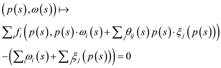
Proof. We consider the mapping 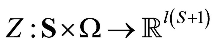 defined by the smooth mapping
 .
.
By the regular value theorem (Guillemin and Pollack [13], p. 21) ![]() is the preimage of
is the preimage of . We need to prove that this mapping does not contain critical points. This follows by showing that the linear tangent map
  is onto. The onto property follows directly from the rank property of the Jacobian matrix chosen for any arbitrary individual
  and state of nature
 . By the chain rule, we obtain
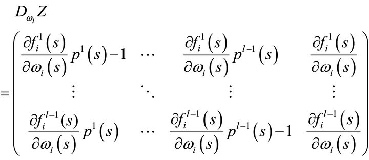
By simple algebraic manipulations we obtain the new matrices

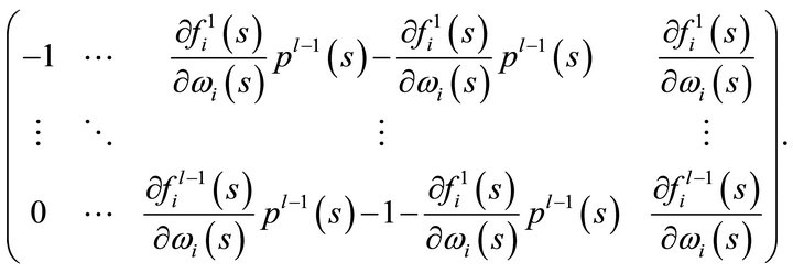
Finally, we obtain

from which we extract the information required. Rank  is equal to
  in every state
 . By the regular value theorem ([13], p. 21)
 ![]() is a smooth manifold. This manifold is parameterized by smooth coordinate functions
is a smooth manifold. This manifold is parameterized by smooth coordinate functions . From the regular value theorem it also follows that its dimension is equal to the dimension of
  minus
minus , hence
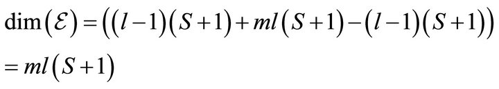 . ■
. ■
The following theorem illustrates a further economically interesting global property of the equilibrium manifold. It says that by construction of a diffeomorphism  restricted to the equilibrium manifold
 ![]() into
into
![]()
 is diffeomorphic to the sphere in
  implying that the equilibrium manifold is arc-connected, simply connected, and contractible. These properties are particularly useful in applied work such as economic policy equilibrium analysis. For example, economic policy is often concerned with finding a path between a current point on
 ![]() and a desired point on
and a desired point on![]() . The following theorem proves that such a path always exists. In order to prove this result, we use a theorem given in (Hirsch [14], pp. 15-16).
. The following theorem proves that such a path always exists. In order to prove this result, we use a theorem given in (Hirsch [14], pp. 15-16).
Theorem 3. The smooth equilibrium manifold ![]() of model
of model  is diffeomorphic to
 .
.
Proof. The aim of the proof is to define two smooth mappings between smooth manifolds such that we can apply the theorem given in (Hirsch [14], pp. 15-16). Hence, let

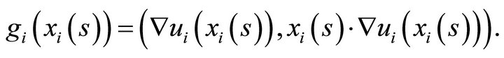
be smooth mappings defined by
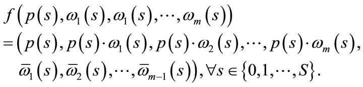
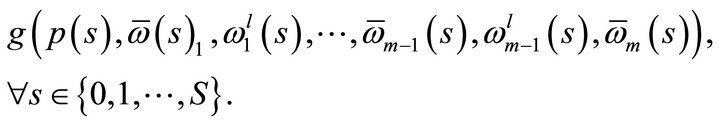
Then, let
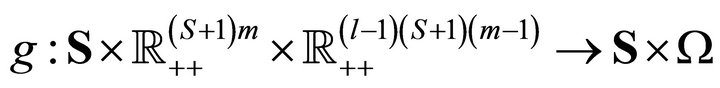
denote smooth mappings defined by
Observe that the coordinates for the  good of the
  consumers in
 ,
,  are defined
 (3)
(3)
Also observe that the coordinates for the  consumer of the
  goods in
 ,
,  are defined by
 (4)
(4)
The application of the theorem in ([14]) requires to show that  and that
 . The first part of the proof requires to calculate two inclusions, 1)
  and 2)
 . We start by showing the second part first. Now, to show that 1)
 , take any consumption bundle
  , and compute the inner product of (4) with
 , and apply Walras’ law to obtain
From that a reformulation of (4) readily follows in terms of the production equilibrium equation
hence . Next, we need to show that 2)
 . Take any arbitrary
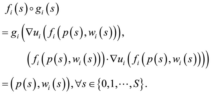
 . It is then trivial to do the computations proving following equality

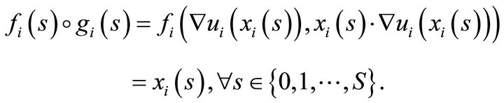
from which it readily follows that . Clearly we have constructed the two smooth relations such that
where  is the identity map defined on
  . We have shown that the smooth mapping f restricted to the equilibrium manifold
 ![]() defines a diffeomorphism between
defines a diffeomorphism between ![]() and the sphere of dimension
and the sphere of dimension . ■
. ■
4. Existence, Efficiency, and Finiteness of Equilibria
We now show that equilibria in the two period production model with uncertainty always exist. The strategy of the proof is to show that the catastrophe mapping  is smooth and proper. Existence of equilibria of this production model with uncertainty follows immediately from the smoothness proposition (1) and the properness proposition (2) below. The result of properness of
 ![]() provides a deep insight into the definition of economics itself. It implies that economic resources are scarce. The diffeomorphism
provides a deep insight into the definition of economics itself. It implies that economic resources are scarce. The diffeomorphism  for all
  between the spaces
  and
and  suggests that the vector
  tends to infinity in norm if prices tend to zero. It tends to zero if prices tend to infinity.
Axiom 4 (Bounded and strictly convex preferences). 1) The set of consumptions bundles indifferent or preferred to consumption bundle  for all
  is bounded from below for every
  for all
 . The preordering
  is then said to be bounded from below; 2) The set of consumptions bundles indifferent or preferred to consumption bundle
  for all
  is strictly convex for every
  for all
  . The preordering
  is then said to be strictly convex.
Theorem 5. Equilibria of the two period production model with uncertainty  always exist.
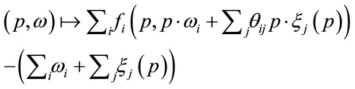
Definition 2. The catastrophe map ![]() is defined by the
is defined by the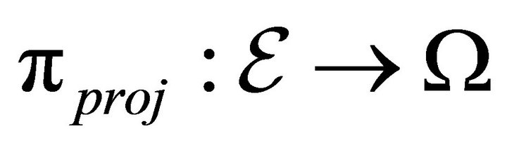 . It is the restriction of the projection
  of the set of equilibria
  into the space of economies
 .
.
Proposition 1 (Smoothness).  of model
  is smooth.
Proof. From Theorem (3) we know that ![]() of model
of model  is a smooth submanifold of
  which is diffeomorphic to the sphere of dimension
 . It follows from the definition of a smooth submanifold ([15], p. 174) that its natural embedding
  is smooth. It is clear that the projection mapping
  is itself smooth. It then follows that
 ![]() the restriction of the natural projection to
the restriction of the natural projection to ![]() as the composition of two smooth mappings
as the composition of two smooth mappings  is therefore smooth. ■
Proposition 2 (Properness).  of model
  is proper.
Proof. The strategy of the proof is to define the economic scenario such that lemma (1) can be applied to the model . Hence, we need to show that for all
  the inverse image
 , where
  is a compact set in the space of initial resources,
  , is compact.
We show that individual consumer demand is bounded below in every uncertain state of the world. To show this, consider any  and define the projection of initial resource into the
  coordinate and state
 ,
,  defined by
Pick an arbitrary  for
for . Let
. Let  be an element in a compact set
 . Note that
  is compact by the projection
  of a compact set
  on the
  coordinate space. Compactness of
  in
in  implies for every
  that
that
1) Now, for every  and
and  and
and  need to show that
  is bounded from below. It then follows from standard assumptions of consumer theory that for all

where
 and
and 
for all .
.
By non satiation we also have

which by monotonicity of  implies that

Clearly, there exists some  for every
  and
and  for all
  satisfying
by boundedness (Axiom 4) of indifference mappings from below for every .
.
2) We now show that for every ,
,  and
and ,
,  is also bounded from above. Consider the equilibrium price vector
  for any
 . Then for all pairs
  we have
where3
Clearly,  , is bounded above by some
 , since for
 is bounded from above for every
 . Hence, we have established the upper and lower bounds for every consumer
  given by
for every .
.
3) We now apply Lemma 1. For any arbitrary consumer , we have established the compact set
 . Let
. Let  be a compact set defined by the preimage of the diffeomorphism
  ([11]) projected onto
 . Hence, we observe that
  is a subset of the compact set
 . Lemma (1) requires to show that
  is closed in
 .
.
Now, by continuity of ,
,  , it follows that
  is closed in
![]() , which by Theorem (1) is a closed subset of
, which by Theorem (1) is a closed subset of . Closedness of
  follows from closedness of
 . ■
. ■
Lemma 2 (Individual demand: Diffeomorphism of ) For every
  the individual demand mapping
  is a diffeomorphism for all
 .
.
Proof. The strategy of the proof is to show that  is smooth, bijective, and that
  is also smooth.
The problem of the consumer is to solve the constraint optimization given by

where
We can use the Lagrangean method to solve this problem. Hence the solution of this problem satisfies the first order conditions of the optmimzation problem and is given by  for all
 . Hence the pair
 , where
  is the Lagrangian multiplier is a solution of the Lagrangian problem. Hence, to show smoothness of
  requires to show that
  is a smooth function of
  and
and . This is a consequence of the implicit function theorem applied to the solutions of the Lagrangian. Hence, we calculate the bordered Hessian matrix,
  for all
 . Thus,

and the inverse of  at
at  exists since
We now show that  is also smooth. Let
  defined by
By assumptions of Debreu [11] all ingredients of this formula are smooth. Also the inner product of smooth functions is smooth. Hence we conclude that  is also smooth.
We now show that  and
and  are inverse mappings for all
 . Hence 1) We calculate the individual composite mapping
  for all
  and show that
 . This condition is satisfied since
As required, we have established
 .
.
2) We calculate the individual composite mapping  for all
  and show that
 . This condition is satisfied since by definition of
  we have
As required, we have established
 . We have proved the bijection property of the individual demand function4. ■
This proves existence of equilibria.
Definition 3. A feasible allocation
![]() associate with equilibrium price vector
associate with equilibrium price vector  and economy
 is Pareto efficient for all
 if there is no other feasible allocation
![]() such that for all
such that for all
 and
and 
with at least one strict inequality.
Theorem 6 (Pareto efficiency of model ). Every economy
  of the model
  is Pareto efficient for all
 .
.
Proof. We proceed by contradiction. We show that if at equilibrium price  the economy
 , where
  is an allocation of consumption and production which is not efficient, then it must be that firms do not maximize profits. This contradicts the assumption that all firms maximize profits (Debreu, [1] Chapter 5) and implies that not all economies are Pareto efficient.
We have for all 
Hence,

Hence we obtain the equilibrium equation given by
We can now establish a contradiction.
Now, let  be an equilibrium price vector for any arbitrary
  and
and  an associated feasible equilibrium allocation which is not Pareto efficient. Since
  is feasible we have
hence
 (5)
(5)
Since by assumption  is not Pareto efficient, there exists a feasible allocation
  associated with with
  and
and  such that

with at least one strict inequality. This implies that
with at least one strict inequality. Aggregating consumption bundles we obtain together with the inner product the strict inequality
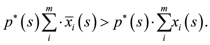 (6)
(6)
Substituting Equation (5) into strict inequality (6) and using the feasible allocation  we obtain
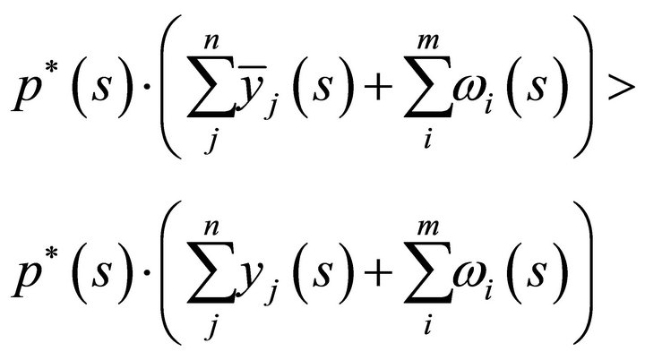
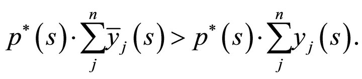
But this strict inequality says that for some  that
that 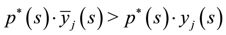 for feasible
 . Hence a violation that firms maximize profits. Clearly, since
  for at least one
 ,
,  is a Pareto inefficient economy. ■
Theorem 7.  of model
  is a finite covering for every
 , for all
 .
.
Proof. Let  consist of a single element of
  for all
 . Consider the tangent map of elements of
 ![]() not contained in the set of singular points,
not contained in the set of singular points, . Then as a non singular point in
 ![]() there exists a bijective map
there exists a bijective map  which by the inverse function theorem implies that
  is locally a diffeomorphism. By the inverse function theorem there exists an open set
  of
of  and an open set
  of
of  such that the restriction of the natural projection to
 ,
,  is a diffeomorphism for all
 . It follows from the one-to-one property of this map that
  . Since
  is open in
 ![]() it follows from the definition of open sets of
it follows from the definition of open sets of  as intersections with
  of open sets of
 ![]() that the subset
that the subset  is open in
 . The union of all open subsets
  define an open covering
  of
of . Compactness of the set
  follows from compactness of the preimage of a compact set
  by the proper mapping
 . It follows from compactness of
  that the open covering has a finite subcovering defined by the unique element of
 . The union of a finite number of elements defines the set
  which is therefore a finite set. This proves finiteness of the number of equilibria. ■
5. Conclusion
This paper discusses local and global equilibrium properties of a production economy with a two period time structure and uncertainty. Adding uncertainty to the production model is a further step towards realism. It is shown that the equilibrium set of all production economies with uncertainty has the structure of a smooth submanifold of the Euclidean space which is diffeomorphic to a sphere. Beyond that, the paper shows that equilibria always exist, and that they are efficient and finite.
REFERENCES
- G. Debreu, “Theory of Value,” New York, Wiley, 1959.
- G. D. K. Arrow, “Existence of an Equilibrium for a Competitive Economy,” Econometrica, Vol. 22, No. 3, 1954, pp. 265-290.
- Y. Balasko, “Economic Equilibrium and Catastrophe Theory: An Introduction,” Journal of Mathematical Economics, Vol. 46, No. 3, 1978, pp. 557-569.
- E. Dierker, “Topological Methods in Walrasian Economics,” Vol. 92, Springer-Verlag, Berlin, 1974. doi:10.1007/978-3-642-65800-6
- Y. Balasko, “The Equilibrium Manifold: Postmodern Developments in the Theory of General Economic Equilibrium,” The MIT Press, Cambridge, 1988.
- E. Jouini, “The Graph of the Walras Correspondence: The Production Economies Case,” Journal of Mathematical Economics, Vol. 22, No. 2, 1993, pp. 139-147.
- G. Fuchs, “Private Ownership Economies with a Nite Number of Equilibria,” Journal of Mathematical Economics, Vol. 1, No. 2, 1974, pp. 141-158.
- S. Smale, “Global Analysis and Econmics IV: Finitness and Stability with General Consumption Sets and Production,” Journal of Mathematical Economics, Vol. 1, No. 2, 1974, pp. 107-117.
- T. Keho, “An Index Theorem for General Equilibrium Models with Production,” Econometrica, Vol. 48, No. 5, 1980, pp. 1211-1232.
- T. Keho, “Regularity and Index Theoy for Econmies with Smooth Production Technologies,” Econometrica, Vol. 51, No. 4, 1983, pp. 895-918.
- G. Debreu, “Smooth Preferences,” Econometrica, Vol. 40, No. 4, 1972, pp. 603-615.
- K. Binmore, “Mathematical Analysis,” 2nd Edition, Cambridge University Press, Melbourne, 1999.
- V. Guillemin and A. Pollack, “Differential Topology,” Prentice Hall, Upper Saddle River, 1974.
- M. Hirsch, “Differential Topology,” Springer, New York, 1972.
- J. Lee, “Introduction to Smooth Manifolds,” Springer, New York, 2000.
NOTES
1Discussion paper: The natural projection approach to smooth production economies, 2011.
2“Smoothness” follows from the assumptions stated in [11]. It essentially means that all functions are differentiable at any order required.
3−i is standard notation used in economic theory. It is equivalent to saying  such that
 , hence
 ![]()
4We have assumed that supply functions are smooth. Hence