Applied Mathematics
Vol. 4 No. 8 (2013) , Article ID: 35484 , 8 pages DOI:10.4236/am.2013.48163
Sobolev Gradient Approach for Huxley and Fisher Models for Gene Propagation
1Department of Mathematics, University of the Punjab, Lahore, Pakistan
2Department of Mathematics and Statistics, McMaster University, Hamilton, Canada
3Department of Mathematics, Lahore University of Management Sciences, Lahore, Pakistan
Email: nraza@math.mcmaster.ca, sultans@lums.edu.pk
Copyright © 2013 Nauman Raza, Sultan Sial. This is an open access article distributed under the Creative Commons Attribution License, which permits unrestricted use, distribution, and reproduction in any medium, provided the original work is properly cited.
Received May 9, 2013; revised June 9, 2013; accepted June 16, 2013
Keywords: Sobolev Gradient; Huxley and Fisher Models; Descent Methods
ABSTRACT
The application of Sobolev gradient methods for finding critical points of the Huxley and Fisher models is demonstrated. A comparison is given between the Euclidean, weighted and unweighted Sobolev gradients. Results are given for the one dimensional Huxley and Fisher models.
1. Introduction
The numerical solution of nonlinear problems is a topic of basic importance in numerical mathematics, as stated in [1]. It has been a subject of extensive investigation in the past decades, thus having vast literature [2-5]. The most widespread way of finding numerical solutions is first discretizing the given problem, then solving the arising system of algebraic equations by a solver which is generally some iterative method. For nonlinear problems most often Newton’s method is used. However, when the work of compiling the Jacobians exceeds the advantage of quadratic convergence, one may prefer gradient type iterations including steepest descent or conjugate gradients. An important example in this respect is the Sobolev gradient technique, which is relying on descent methods. The Sobolev gradient technique presents a general efficient preconditioning approach where the preconditioners are derived from the representation of the Sobolev inner product.
Sobolev gradients have been used for ODE problems [6,7] in a finite-difference setting, PDEs in finite-difference [7,8] and finite-element settings [9], minimizing energy functionals associated with Ginzburg-Landau models in finite-difference [10] and finite-element [11,12] settings and related time evolutions [13], the electrostatic potential equation [1], nonlinear elliptic problems [14], semilinear elliptic systems [15], simulation of Bose-Einstein condensates [16], inverse problems in elasticity [17] and groundwater modelling [18].
A detailed analysis regarding the construction and the application of Sobolev gradients can be found in [6]. For a quick overview of Sobolev gradients, applications and some open problems in the subject we refer to [19].
Sobolev gradients are also useful for preconditioning for linear and nonlinear problems. Sobolev preconditioning [20] has been tested on some first order and second order linear and nonlinear problems and it is found comparable in terms of efficiency and stability with other methods such as Newton’s method and Jacobi method. For differential equations with nonuniform behavior on long intervals, “Sobolev gradients have proved to be effective if we divide the interval of interest into pieces and take a recursive approach (cf. [21])”. Sobolev gradients have interesting applications in the field of geometric modelling [22]. It has been proved therein that the Sobolev gradient is a very useful tool for minimizing functionals that pertain to the length of curves, curvatures, surface area etc. Recently, the paper [23] has shown the possible applications of Sobolev gradient technique for systems of Differential Algebraic Equations.
The idea of a weighted Sobolev gradient has been introduced by W. T. Mahavier in [7]. The weighted Sobolev gradient has successfully exhibited its effectiveness in dealing with linear and nonlinear singular differential equations with regular and some typically irregular singularities. Weighted gradients have also been used for DAEs and it turns out that weighted Sobolev gradients outperform unweighted Sobolev gradients in many situations.
In the field of gene technolog, Modelling of gene frequencies is of the prospective area of research. Its applications can be seen in livestocks and agricultural crops. By the modification of their genes, they can be made more resistive to infection and to produce more yield. To derive historical patterns of migration, archaeologists are expecting that study of the entire human genetic material, will facilitate to map geographical distribution of signature genes. By using gene technology, many bacteria have been developed to prescribed antibiotics. From medical point of view, it is important to study the genetic background of diseases, with implications in diagnosis, treatment and drug development. In order to make use of genetic population data, we need to understand the dynamics of gene patterns through the population.
2. Fisher and Huxley Models
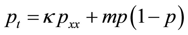
In the 1930s, number of authors proposed reaction-diffusion equations to model changing gene frequencies in a population. One of the earliest and best known such equations was that of Fisher. In his paper in 1937 [24], he proposed a reaction-diffusion equation with quadratic source term that models the spread of a recessive advantageous gene through a population i.e.;
 (1)
(1)
where ![]() is the frequency of the new mutant gene,
is the frequency of the new mutant gene, ![]() is the coefficient of diffusion, and
is the coefficient of diffusion, and ![]() is the intensity of selection in favor of the mutant gene. The equation predicts a wave front of increasing allele frequency, propagating through a population. The quadratic logistic term of Fisher’s equation is more appropriate for asexual species.
is the intensity of selection in favor of the mutant gene. The equation predicts a wave front of increasing allele frequency, propagating through a population. The quadratic logistic term of Fisher’s equation is more appropriate for asexual species.
Fisher’s assumptions for a sexually reproducing species lead to a Huxley reaction-diffusion equation, with cubic logistic source term for the gene frequency of a mutant advantageous recessive gene. Huxley’s equation is given by
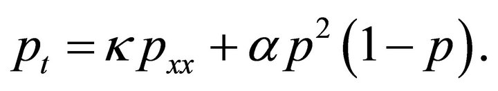 (2)
(2)
3. Review of Sobolev Gradient Methods
In this section we discuss the Sobolev gradient and steepest descent. A detailed analysis regarding the construction of Sobolev gradients can be seen in [6].
Let us consider ![]() is a positive integer and
is a positive integer and  is a real valued
  function on
 . We can define its gradient
  as
as
 (3)
(3)
For  as above, but with
  an inner product on
  different from the standard inner product
 , there is a function
  so that
 (4)
(4)
The linear functional  can be represented using any inner product on
 . Let us call
  is the gradient of
  with respect to the inner product
  and it can be seen that
  has the same properties as
 .
.
By applying a linear transformation, we have
 we can relate these two inner products

for , and by a reflection
 (5)
(5)
For each  an inner product is assciated
on . Thus for
 , define
  such that
 (6)
(6)
When gradient is defined in a finite or infinite dimensional Sobolev space we call it Sobolev gradient. Steepest descent can be classified into two categories: the one is discrete and other continuous steepest descent. Let  be a real-valued
  function, defined on a Hilbert space
  and
and  be its gradient with respect to the inner product
  defined on
 . Discrete steepest descent method is a process of constructing a sequence
  so that
  is given and
 (7)
(7)
where for each ,
,  is chosen so that
 (8)
(8)
is minimal in some appropriate sense. In continuous steepest descent we construct a function  so that
 (9)
(9)
Under suitable conditions on ,
,  where
where  is the minimum value of
 .
.
Continuous steepest descent is interpreted as a limiting case of discrete steepest descent. So (7) can be considered as a numerical method for approximating solutions to (9). Continuous steepest descent gives a theoretical starting point for proving convergence of discrete steepest descent. Using (7) one seeks  , so that
 (10)
(10)
and using (9) one seeks  so that (10) holds. Two groups of problems can be cast in terms of determining the functional
 . The first group deals with those problems where
  serves as an energy functional. For cases of the use of
  as an energy functional see [6,10,12,13].
Now we solve these problems by using various descent techniques.
3.1. Using Second Order Operators
Consider Fisher’s equation
 (11)
(11)
in the space domain  which is the interval [0,2]. We use Neumann boundary conditions, i.e.
 .
.
Now a suitable finite difference discretization will be done. We work with a finite-dimensional vector  on the interval. We will denote by
  the vector space
  equipped with the usual inner product
 . The operators
 are defined by
 (12)
(12)
 (13)
(13)
 (14)
(14)
for  and where
  is the spacing between the nodes.
  just picks up the points in the grid which are not on the endpoints.
  and
and  are standard central difference formulas for estimating the first and second derivatives. The choice of difference formula is not central to the theoretical development in this paper, other choices would also work. The numerical version of the problem of evolving from one time
  to a time
  is to solve
 (15)
(15)
where  in the equation is
 ![]() at the previous time and
at the previous time and ![]() is the
is the ![]() desired at the next time level. In terms of operators problem can be written as
desired at the next time level. In terms of operators problem can be written as
 (16)
(16)
The time-step  must be prescribed small enough ti have
 . We can put the solution of this problem in other terms of minimizing a functional via steepest descent. Define
  by
by
 (17)
(17)
which is zero when the we have the desired![]() . The functional
. The functional
 (18)
(18)
has a minimum of zero when  is zero so we will look for the minimum of this functional. This functional is a convex functional that guarantees global minima in
 , a solution to problem (11). The aim is to find the gradient of a convex functional
  associated with the problem and use this gradient in steepest descent minimization process to finding the zero of the functional, that is the minimum of
  and the solution of the original problem.
3.2. Gradients and Minimization
The gradient  of a functional
  in
in  is found by solving
 (19)
(19)
for test function . The gradient points in the direction of greatest increase of the functional. The direction of greatest decrease of the functional is
 . This is the basis of steepest descent algorithms. One can reduce
  by replacing an initial
 ![]() with
with  where the step size
 ![]() is a positive number. This can be done repeatedly until either
is a positive number. This can be done repeatedly until either  or
or  is less than some specified tolerance. We desire a finitedimensional analogue to the original problem in which
  on the endpoints of the interval. So, we use a projection
  which projects vectors in
  onto the subspace in which the gradient vanishes at the boundary. Rather than using
 , we will use
 . The steepest descent algorithm in this new space now looks like 1) Calculate
 ;
;
2) Update ![]() by
by  where
where ![]() is some fixed positive number;
is some fixed positive number;
3) Repeat.
In this particular case,
 (20)
(20)
gives the desired gradient for steepest descent in . The operators
  are the adjoints of
  and
and  respectively. The Sobolev gradient approach to the problem of minimizing functionals is to do the minimization in Sobolev spaces which correspond to the problem. In this paper only discrete Sobolev spaces are used. We define two such spaces in which the minimization can be compared to minimization in
 . We are prompted to consider the space
  which is
  with the inner product
 (21)
(21)
because  and
and  have
have  in them. We also follow the technique of Mahavier for solving differential equations for this we define a new inner product
  as
as  equipped with the inner product
 (22)
(22)
because this takes into account the coefficients of  and
and  in
in  and
and . The desired Sobolev gradients
 ,
,  in
in  and
and  are found by solving
 (23)
(23)
 (24)
(24)
respectively. Here  is the adjoint of
 . Following the same line we construct the gradients for Huxley’s model.
Numerical experiments for the solution of Fisher and Huxley’s equations were conducted as follows. A system of  nodes was set up with
  i.e. the initial conditions. The internodal spacing was
 . The value of
 ![]() was set to 1 for all the experiments. We chose
was set to 1 for all the experiments. We chose  with
with  so that both source functions has the same maximum value. The function
 ![]() was then evolved. The updated value of
was then evolved. The updated value of ![]() for a given time step was considered to be correct when the infinity norm of
for a given time step was considered to be correct when the infinity norm of  was less than
![]() . We set
. We set  for the time increment. For the gradients in
  and
and  we used the same step size regardless of the nodal spacing. The total number of minimization steps for fifteen time steps, the largest value of
 ![]() that can be used and CPU time were recorded in Tables 1 and 2.
that can be used and CPU time were recorded in Tables 1 and 2.
From the tables we see that the results in  are far better than
 , in fact there is no
  convergence for
 . The best results are in the weighted Sobolev space
 . When we perform minimization in
  the convergence is three times faster for solving Huxley’s model than from that
 .
.
3.3. Using the Associated Functional
Here we suggest another approach, in order to avoid second order operators. Once again consider the problem
 (25)
(25)
with Neumann boundary conditions. We think of the  nodes as dividing up [0,2] into
  subintervals. The
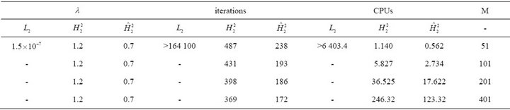
Table 1. Numerical results of steepest descent in ,
,  ,
,  using
using  over
over  time steps using second order operators for Fisher’s model.

Table 2. Numerical results of steepest descent in ,
,  ,
,  using
using  over
over  time steps using second order operators for Huxley’s model.
operators  estimates
 ![]() on the interval by
on the interval by
 (26)
(26)
for .
.  estimates the first derivative on the intervals by
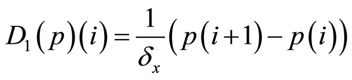 (27)
(27)
for  and where
  is the internodal spacing. The associated functional for a finite dimensional version of the problem with discrete time steps is given by
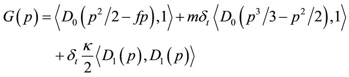 (28)
(28)
and we wish to minimize the functional  until
until  is smaller than some set tolerance.
  has a minimum when the gradient
 (29)
(29)
is equal to zero, and this might be considered the condition for finding ![]() at the next time step. Here
at the next time step. Here  are the adjoins of
  respectively. We want to minimize this functional in
 and also in some new inner product spaces
 ,
,  , defined via
 (30)
(30)
 (31)
(31)
Once again numerical experiments are conducted by using the same parameters as defined earlier. for solution of Fisher and Huxley models were conducted as follows. The updated value of ![]() for a given time step was considered to be correct when the infinity norm of
for a given time step was considered to be correct when the infinity norm of  was less than
![]() . We set
. We set  for the time increment. For the gradients in
  and
and  we used the same step-size regardless of the nodal spacing. The total number of minimization steps for fifteen time steps, the largest value of
 ![]() that can be used and CPU time were recorded in Tables 3 and 4.
that can be used and CPU time were recorded in Tables 3 and 4.
We note that the finer the spacing the less CPU time the Sobolev gradient technique uses in comparison to the usual steepest descent method. The step size for minimization in  has to decrease as the spacing is refined. From the tables one can see that the results in
  are far better than
  and results in the space
  are the best.
3.4. Using First Order Operators
Once again consider the problem
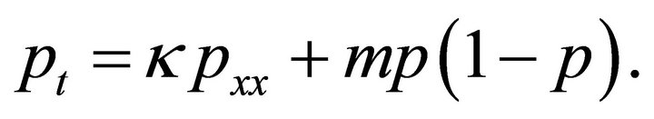
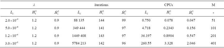
Table 3. Numerical results of steepest descent in ,
,  ,
,  using
using  over 15 time steps using the associated functional for the Fisher’s model.
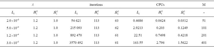
Table 4. Numerical results of steepest descent in ,
,  ,
,  using
using  over
over  time steps using the associated functional for the Huxley’s model.
Let us write this as a system of two equations
 (32)
(32)
 (33)
(33)
A finite-dimensional version which is first order in time is to solve
 (34)
(34)
 (35)
(35)
We define functions
 (36)
(36)
 (37)
(37)
The functional for the problem is
 (38)
(38)
The problem is considered to be solved when  has been minimized, that is, when
  or infinity norms of
 ![]() and
and ![]() are less than some desired tolerance. The
are less than some desired tolerance. The  gradients are
 (39)
(39)
 (40)
(40)
The Sobolev gradients in  are found by solving
 (41)
(41)
 (42)
(42)
We want to minimize this functional in ,
,  and also in the new inner product spaces
  and
and . To define these new inner products we follow the technique of Mahavier [7] for singular differential equations and use weighted Sobolev spaces
  and
and  such that
 (43)
(43)
 (44)
(44)
and new gradients  are found by solving
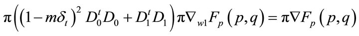 (45)
(45)
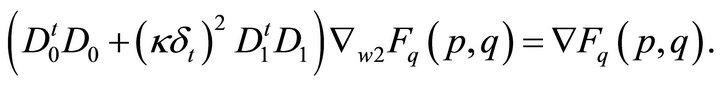 (46)
(46)
Numerical experiments are conducted by using the same parameters as defined in Section . The updated value of
 ![]() for a given time step was considered to be correct when the infinity norms of both
for a given time step was considered to be correct when the infinity norms of both ![]() and
and ![]() were less than
were less than![]() . We set
. We set  for the time increment. The total number of minimization steps for fifteen time steps, the largest value of
 ![]() that can be used and CPU time were recorded in Tables 5 and 6.
that can be used and CPU time were recorded in Tables 5 and 6.
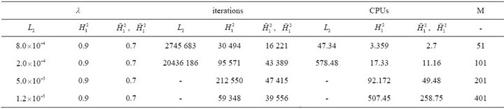
Table 5. Numerical results of steepest descent in ,
,  and
and ,
,  using
using  over 15 time steps using first order operators for the Fisher’s model.
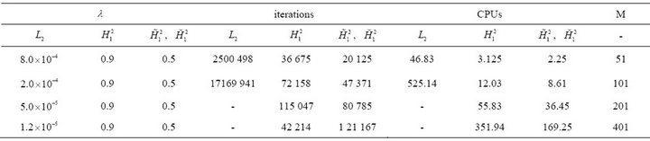
Table 6. Numerical results of steepest descent in ,
,  and
and ,
,  using
using  over 15 time steps using first order operators for the Huxley’s model.
We note that the finer the spacing the less CPU time the Sobolev gradient technique uses in comparison to the usual steepest descent. For the Fisher and Huxley model the same step size ![]() can be used for all spacings
can be used for all spacings ![]() when minimizing in the appropriate Sobolev space. The step-size for minimization in
when minimizing in the appropriate Sobolev space. The step-size for minimization in  has to decrease as the spacing is refined.
From the table one can see that the results in  are far better than
  and results in the space
 ,
,  are the best.
4. Summary and Conclusions
In this paper, we have presented minimization schemes for the Huxley and Fisher’s models based on the Sobolev gradient technique [6]. The Sobolev gradient technique is computationally more efficient than the usual steepest descent method as the spacing of the numerical grid is made finer. Choosing an optimal inner product can improve the performance with respect to which the Sobolev gradient works better. it is still an open question what the absolutely optimal inner product is, and it is possible that different inner products might not make large differences in computational performance in all cases. One advantage of steepest descent is that it converges even for a poor initial guess. The Sobolev gradient methods presented here converge even for rough initial guess or jumps in the initial guess.
In Figures 1 and 2, we display the numerical solution of two models with the same localized Gaussian clump of the mutant alleles, contained within the region  by zero flux boundary conditions i.e.;
 .
.
We choose  with
with  and diffusion coefficient
  so that the differences in the source term can be highlighted in comparison to the diffusion
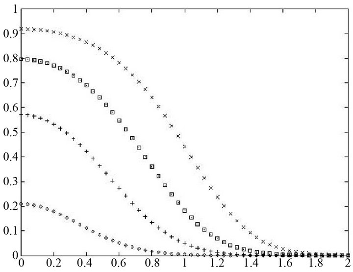
Figure 1. Graph of solution of Fisher’s equation for t = 0.1, 3, 5, 7.

Figure 2. Graph of solution of Huxley’s equation for t = 0.1, 5, 10, 20, 30, 37.
effects. For both models the mutant gene frequency can be seen to increase at the origin and then spread throughout the range. As expected mutant take over is greatly retarded in the Huxley model compared to the Fisher model. So, for asexually reproducing population, a cubic source term is more appropriate than a quadratic source term and for sexually reproducing population, Fisher’s equation is more appropriate.
REFERENCES
- J. Karatson and L. Loczi, “Sobolev Gradient Preconditioning for the Electrostatic Potential Equation,” Computers & Mathematics with Applications, Vol. 50, No. 7, 2005, pp. 1093-1104. doi:10.1016/j.camwa.2005.08.011
- R. Glowinski, “Numerical Methods for Nonlinear Variational Problems,” Springer-Verlag, New York, 1997.
- A. Zenisek, “Nonlinear Elliptic and Evolution Problems and Their Finite Element Approximations,” Academic Press, London, 1990.
- I. Farago and J. Karatson, “Numerical Solution of Nonlinear Elliptic Problems via Preconditioning Operators,” Advances in Computation, Vol. II, Nova Science Publishers, New York, 2002.
- C. T. Kelley, “Iterative Methods for Linear and Nonlinear Equations,” SIAM: Frontiers in Applied Mathematics, Philadelphia, 1995.
- J. W. Neuberger, “Sobolev Gradients and Differential Equations,” Springer Lecture Notes in Mathematics 1670, Springer-Verlag, New York, 1997.
- W. T. Mahavier, “A Numerical Method Utilizing Weighted Sobolev Descent to Solve Singluar Differential Equations,” Nonlinear World, Vol. 4, No. 4, 1997, pp. 435-455.
- D. Mujeeb, J. W. Neuberger and S. Sial, “Recursive form of Sobolev Gradient Method for ODEs on Long Intervals,” International Journal of Computer Mathematics, Vol. 85, No. 11, 2008, pp. 1727-1740. doi:10.1080/00207160701558465
- C. Beasley, “Finite Element Solution to Nonlinear Partial Differential Equations,” PhD Thesis, University of North Texas, Denton, 1981.
- S. Sial, J. Neuberger, T. Lookman and A. Saxena, “Energy Minimization Using Sobolev Gradients: Application to Phase Separation and Ordering,” Journal of Computational Physics, Vol. 189, No. 1, 2003, pp. 88-97. doi:10.1016/S0021-9991(03)00202-X
- S. Sial, J. Neuberger, T. Lookman and A. Saxena, “Energy Minimization Using Sobolev Gradients Finite Element Setting,” Proceedings of World Conference on 21st Century Mathematics, Lahore, 4-6 March 2005, pp. 234- 243.
- S. Sial, “Sobolev Gradient Algorithm for Minimum Energy States of s-Wave Superconductors: Finite Element Setting,” Superconductor Science and Technology, Vol. 18, No. 5, 2005, pp. 675-677. doi:10.1088/0953-2048/18/5/015
- N. Raza, S. Sial and S. S. Siddiqi, “Sobolev Gradient Approach for the Time Evolution Related to Energy Minimization of Ginzberg-Landau Energy Functionals,” Journal of Computational Physics, Vol. 228, No. 7, 2009, pp. 2566-2571. doi:10.1016/j.jcp.2008.12.017
- J. Karatson and I. Farago, “Preconditioning Operators and Sobolev Gradients for Nonlinear Elliptic Problems,” Computers & Mathematics with Applications, Vol. 50, No. 7, 2005, pp. 1077-1092. doi:10.1016/j.camwa.2005.08.010
- J. Karatson, “Constructive Sobolev Gradient Preconditioning for Semilinear Elliptic Systems,” Electronic Journal of Differential Equations, Vol. 75, No. 1, 200, pp. 1- 26.
- J. Garcia-Ripoll, V. Konotop, B. Malomed and V. PerezGarcia, “A Quasi-Local Gross-Pitaevskii Equation for Attractive Bose-Einstein Condensates,” Mathematics and Computers in Simulation, Vol. 62, No. 1-2, 2003, pp. 21- 30. doi:10.1016/S0378-4754(02)00190-8
- B. Brown, M. Jais and I. Knowles, “A Variational Approach to an Elastic Inverse Problem,” Inverse Problems, Vol. 21, No. 6, 2005, pp. 1953-1973. doi:10.1088/0266-5611/21/6/010
- I. Knowles and A. Yan, “On the Recovery of Transport Parameters in Groundwater Modelling,” Journal of Computational and Applied Mathematics, Vol. 71, No. 1-2, 2004, pp. 277-290. doi:10.1016/j.cam.2004.01.038
- R. J. Renka and J. W. Neuberger, “Sobolev Gradients: Introduction, Applications,” Contmporary Mathematics, Vol. 257, 2004, pp. 85-99.
- W. B. Richardson, “Sobolev Preconditioning for the Poisson-Boltzman Equation,” Computer Methods in Applied Mechanics and Engineering, Vol. 181, No. 4, 2000, pp. 425-436. doi:10.1016/S0045-7825(99)00182-6
- D. Mujeeb, J. W. Neuberger and S. Sial, “Recursive Forms of Sobolev Gradient for ODEs on Long Intervals,” International Journal of Computer Mathematics, Vol. 85, No. 11, 2008, pp. 1727-1740. doi:10.1080/00207160701558465
- R. J. Renka, “Geometric Curve Modeling with Sobolev Gradients,” 2006. www.cse.unt.edu/renka/papers/curves.pdf
- R. Nittka and M. Sauter, “Sobolev Gradients for Differential Algebraic Equations,” Journal of Differential Equations, Vol. 42, No. 1, 2008, pp. 1-31.
- R. A. Fisher, “The Wave of Advance of Advantageous Genes,” Annals of Eugenics, Vol. 7, No. 4, 1937, pp. 355- 369. doi:10.1111/j.1469-1809.1937.tb02153.x
- R. Courant, K. O. Friedrichs and H. Lewy, “Uber die Partiellen Differenzengleichungen der Mathematisches Physik,” Mathematische Annalen, Vol. 100, No. 1, 1928, pp. 32-74. doi:10.1007/BF01448839