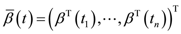
Applied Mathematics
Vol.4 No.5(2013), Article ID:31572,5 pages DOI:10.4236/am.2013.45117
Local Influence Analysis of Varying-Coefficient Model with Random Right Censorship
Department of Fundamental Course, Air Force Logistics College, Xuzhou, China
Email: wangshuling2007@yahoo.com.cn
Copyright © 2013 Shuling Wang et al. This is an open access article distributed under the Creative Commons Attribution License, which permits unrestricted use, distribution, and reproduction in any medium, provided the original work is properly cited.
Received October 19, 2012; revised April 3, 2013; accepted April 10, 2013
Keywords: Random Right Censorship; B Splines; Local Influence
ABSTRACT
For this model, this paper studies the method and application of the diagnostic mostly. Firstly, the primary model is transformed to varying-coefficient model by using a general transformation method. Secondly, a simple estimation form of the coefficient functions is obtained by employing the B spline. Then, local influence is discussed and concise influence matrix is obtained. At last, an example is given to illustrate our results.
1. Introduction
Local influence analysis is proposed from the viewpoint of differential geometry [1]. Nearly thirty years, the diagnosis and influence analysis of linear regression model have been fully developed (Ref. [2,3]). The varing-coefficient model is a useful extension of classical linear model. It has been widely applied in statistical modelling, for example, see Ref. [1,4-6]. However, all the above results are obtained under the uncensored case. In many applications, some of the responses and/or covariates may not be observed, but are censored. For censored data, the usual statistical techniques for complete data situations are not readily applicable. When the response is censored, the relationship between the response and the covariate has been widely studied in the literature [7-10].
So far the local influence analysis of varying-coefficient model with random right censorship has not yet seen in the literature, this paper attempts to study it. The paper is organized as follows: The introduction of local influence is given in Section 2; The model and the estimators are introduced in Section 3; The statistical diagnostics are given in Section 4; The example to illustrate our results is given in Section 5.
2. Local Influence
Ref. [2,3] have discussed the method of local influence analysis. Let  be an unknown k-dimensional parameter, whose domain is an open subset of Euclidean space
 .
.  is a object function (for example, likelihood function, punishment log-likelihood function).
 ![]() is a n-vector which denotes disturbed factor, for example weighted or tiny shift. Let
is a n-vector which denotes disturbed factor, for example weighted or tiny shift. Let  be the disturbed model, whose object function is
 .
.  is the estimate which is from
 . Given
  makes
makes  and
and , where
  has continuous second-order partial derivatives,
  is the function of
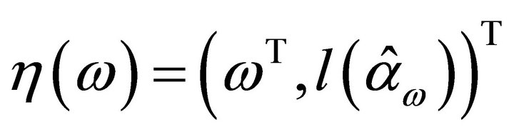
![]() . In geometry,
. In geometry,  denotes n-dimentional surface
 (1)
(1)
This image is called influence image, which varies with![]() . The variation rate in
. The variation rate in  of influence image reflects that the sensitivity of model, where
  corresponds to the primary model. This method is called local influence. COOK advanced that utilize influence curvature to measure the change of influence image near
 .
.
Ref. [2,3] pointed out that the influence curvature of 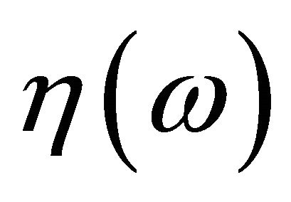 is given by
 (2)
(2)
where  is second derivatives of
  with respect to
![]() , and
, and
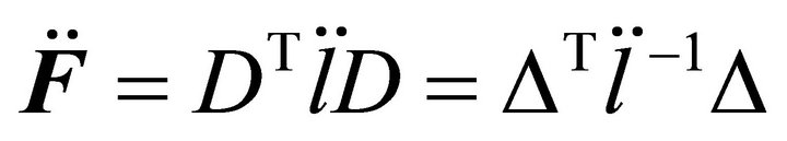
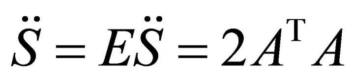
 (3)
(3)
D and  are
are  matrix, where
 .
.
The influence matrix is given by
 (4)
(4)
Formula (2) shows that the maximal influence curvature , where
  is the eigenvalue of
  whose absolute value is maximal, and
 ![]() is the corresponding eigenvector which is called the direction of maximal influence curvature. Ref. [5] pointed out that the diagonal value of influence matrix also is the important diagnostic statistics.
is the corresponding eigenvector which is called the direction of maximal influence curvature. Ref. [5] pointed out that the diagonal value of influence matrix also is the important diagnostic statistics.
3. The Model and Estimators
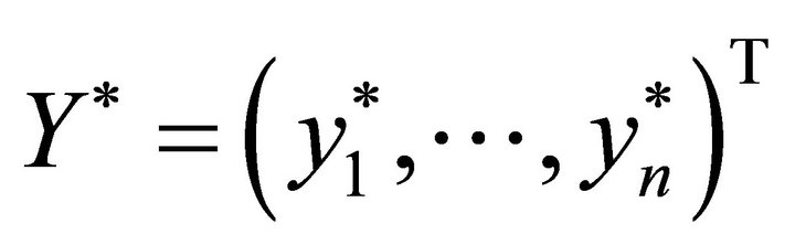
Let Y be the response variable and  be its associated covariates. The varying-coefficient regression model assumes the following structure:
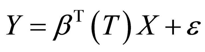 (5)
(5)
where 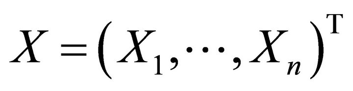 is of dimension
 ![]() and
and
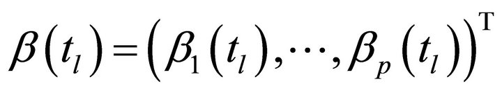
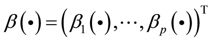 is a p-dimensional vector of unknown coefficient functions.
 ![]() is a stochastic error with
is a stochastic error with
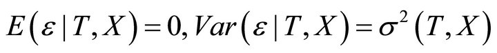 .
.
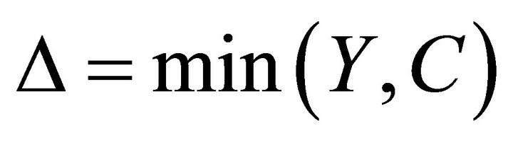
Consider the model (5), where Y is the survival time. Let C be the censoring time associated with the survival time Y. Assume that Y and C are conditionally independent given the associate covariates . Denote
 and
and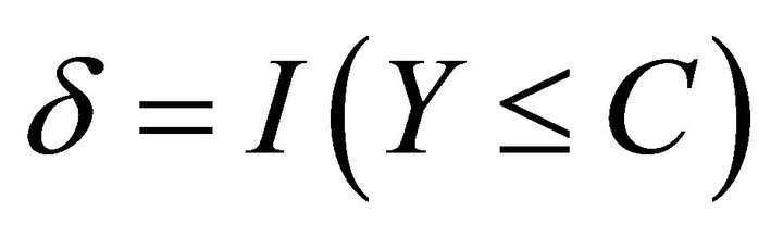 , where
  is the index function. The observations are
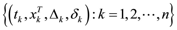 which are random samples from
 , where
 . Thus instead of observing
 , we observe the pairs
 , where
 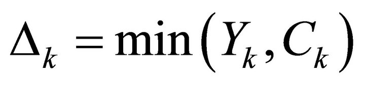 and
and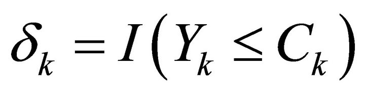 . Observations on
  for which
  are uncensored, and observations on
  for which
  are censored. Model (5) is called varying-coefficient regression model with random right censorship right now. Let
  is the distribution function of
![]() , G is the common distribution function of
, G is the common distribution function of , and
, and . Note that
  and
and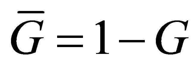 .
.
Lemma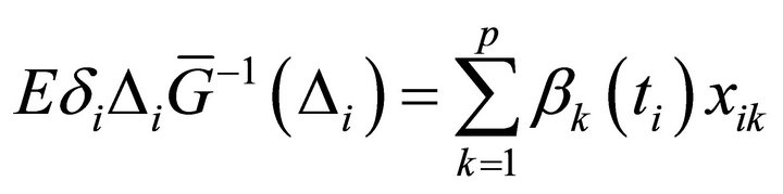 ,
, .
.
Proof. Since
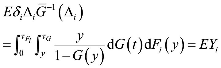
and
thus ,
, .
.
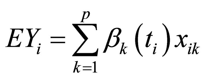
Now we consider  follow the model
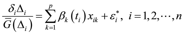 (6)
(6)
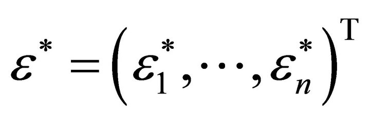
where  is i.i.d. and
 ,
, . In practice, we replace
  with
with  which is the KaplanMeier product-limited estimator of
  (Ref. [11]). The expression of
  is given as follows:
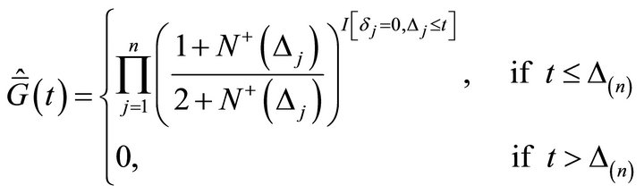 (7)
(7)
where 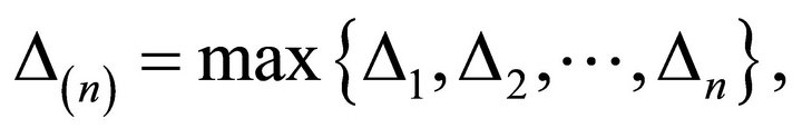
![]() .
.
Let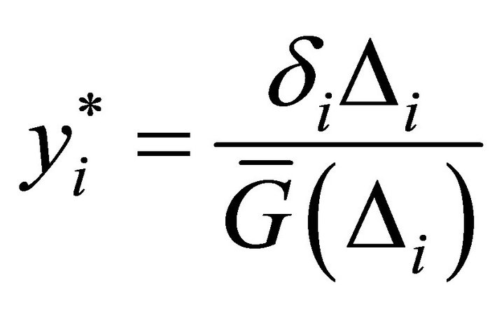 , model (5) is transformed to following varying-coefficient regression model
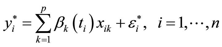 (8)
(8)
Now we want to estimate the unknown coefficient function vector based on the transformed data. In varying-coefficient model, there are a lot of estimates for . Here we use the B-spline estimate
 .
.
Let  are the knots in
 ,
,  and
and 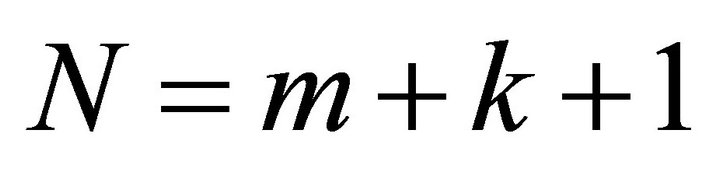 are the basis functions of m-th B-spline,
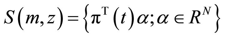 is the space of m-th Bspline function. We use the lemma 1.2 of Ref. [3], every smooth coefficient function
  can be approximated by B-spline function
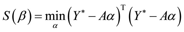
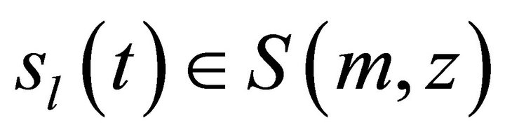 . The B-spline estimator of the coefficient function
 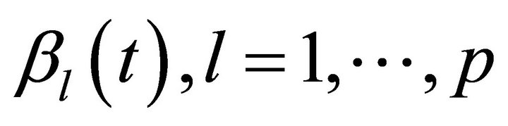 in model (8) is the solution of following formula
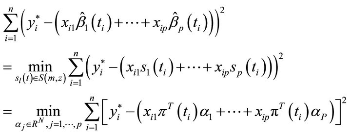 (9)
(9)
In order to depict conveniently, supposed that
 ,
,  ,
,
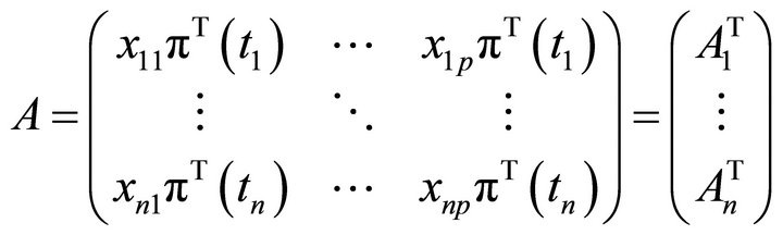 ,
,
 ,
,  ,
,
 ,
,  ,
,
 ,
,
 then
then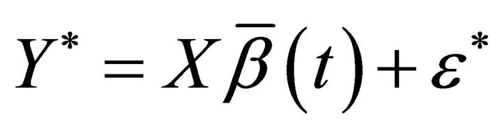 , and Formula (9) can be transformed to following minimize problem
 (10)
(10)
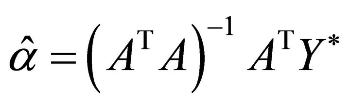
Utilize the least-square method, the estimator of ![]() is
is
The estimator of the l-th coefficient function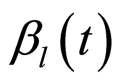 ,
,  is
is
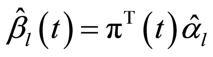
Then, the estimator of the coefficient function  is
is
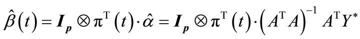 (11)
(11)
where  is an
is an  unit matrix, and
 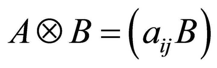 is Kronecker product of matrix.
4. The Local Influence of the Model
4.1. Weighted Perturbation Model
Suppose that , then the weighted perturbation model can be shown that
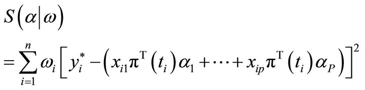 (12)
(12)
Substituting this result into (3) yields
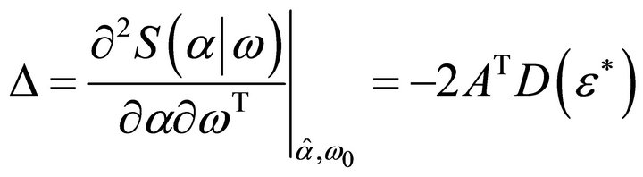 (13)
(13)
where 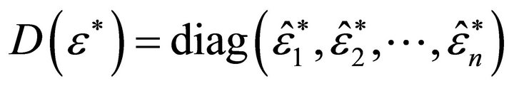 and
and the second derivatives of
  with respect to
 ![]()
is given by
 (14)
(14)
Substituting (13) and (14) into (4), we obtain the corresponding influence matrix
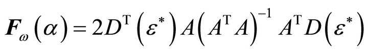 (15)
(15)
Here 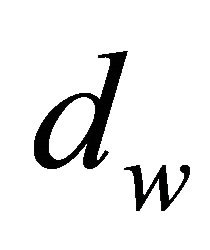 denotes the direction of maximal influence curvature.
4.2. Response Variable Perturbation Model
Suppose that , then the response variable perturbation model can be shown that
 (16)
(16)
Substituting this result into (3) yields
 (17)
(17)
the second derivatives of  with respect to
 ![]() is given by
is given by
 (18)
(18)
Substituting (17) and (18) into (4), we obtain the corresponding influence matrix
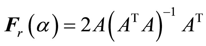 (19)
(19)
Here  denotes the direction of maximal influence curvature.
5. An Illustrative Example
(Vicious Tumour Data) Now we consider an example as the illustration for the above results. Considering a clinical research trial data (see Ref. [4]), there are 205 cancer patients who have been treated in Odense university hospital and tracked until the end of 1977. The survival time of some individuals due to death or end of the trial for other reasons were censored. Ref. [11] utilized a linear semi-parametric model to fit this test data. We utilized varying-coefficient model to fit the data of 57 patients. Where  denoted the thickness of tumour,
 ![]() denoted the sex (1 is male, 0 is female). Considering that there was
denoted the sex (1 is male, 0 is female). Considering that there was
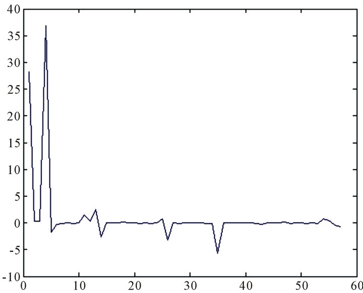
Figure 1. The direction of maximal influence curvature dwj.
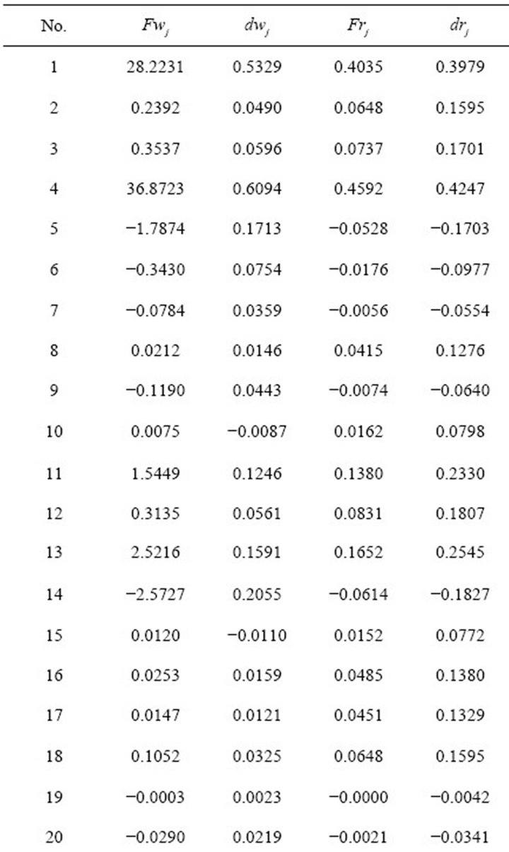
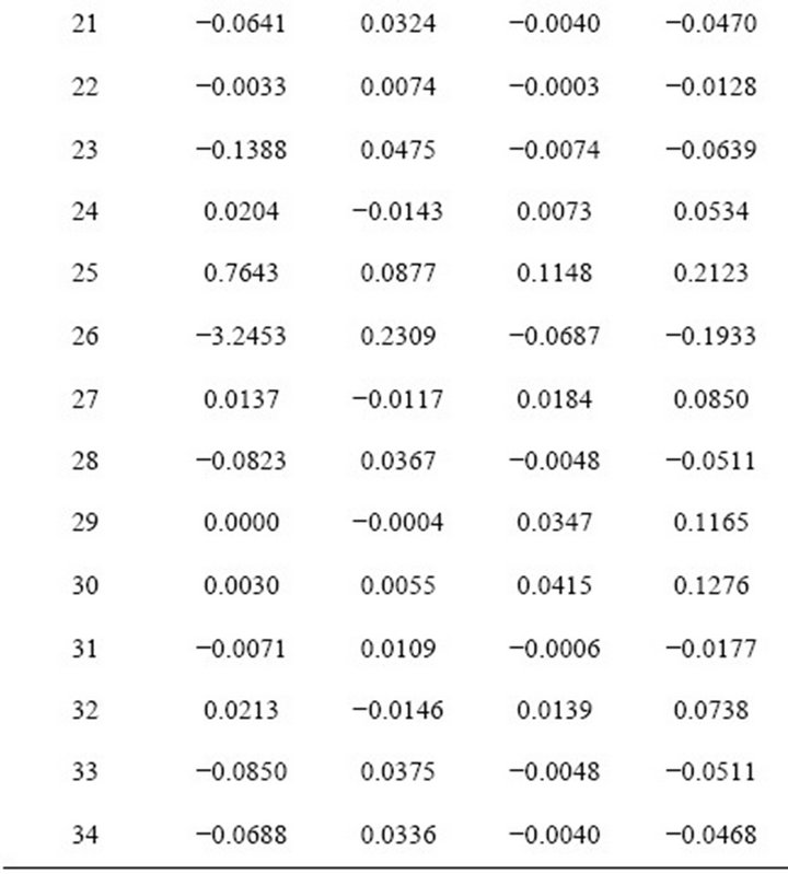
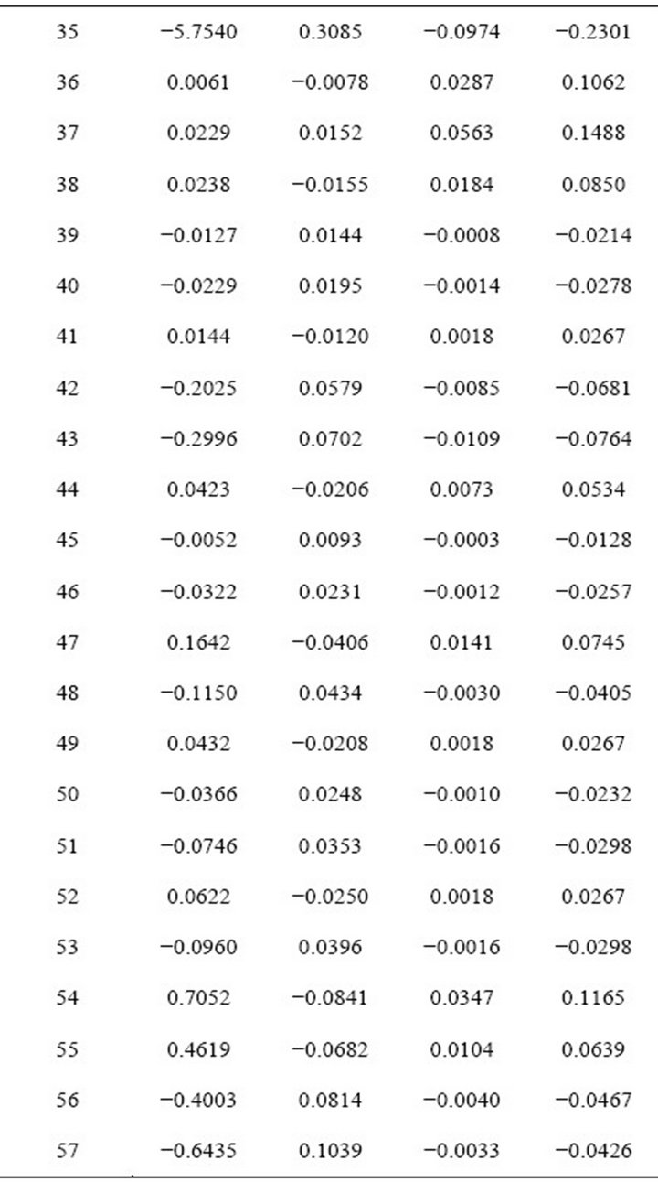
Table 1. The value of static.
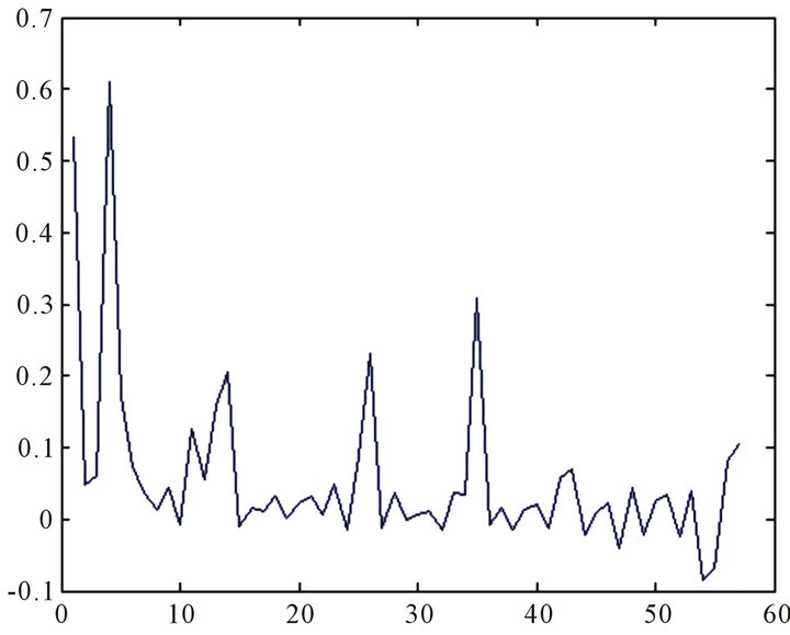
Figure 2. The diagonal value of influence matrix Fwj.
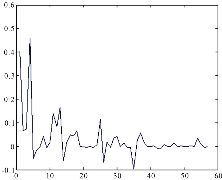
Figure 3. The diagonal value of influence matrix Frj.
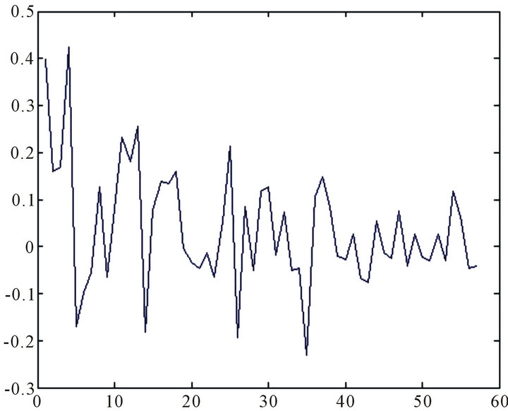
Figure 4. The direction of maximal influence curvature drj.
relation between the thickness of tumor and the sex, so we supposed that there was a relation between the coefficient 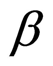 and
and![]() . Hence, we utilized the varying-coefficient model
. Hence, we utilized the varying-coefficient model  to analyze these data. The results are as Table 1 and Figures 1-4.
Figures 1 and 2 show that the first and the fourth data are the outlier, Figures 3 and 4 show that the first and the fourth data are the outliers. Indeed, the diagnostic effect of the diagonal value is identical with the direction of maximal influence curvature and this result is similar to Li Yali [12].
REFERENCES
- R. D. Cook, “Assessment of Local Influence (with Discussion),” Journal of the Royal Statistical Society: Series B, Vol. 48, No. 2, 1986, pp. 133-169.
- R. D. Cook and S. Weisberg, “Residuals and Influence in Regression,” Chapman and Hall, New York, 1982.
- B. C. Wei, G. B. Lu and J. Q. Shi, “Statistical Diagnostics,” Publishing House of Southeast University, Nanjing, 1990.
- P. K. Andersen, O. Borgan, R. D. Gill and N. Keiding, “Statistical Models Based on Counting Processes,” SpringerVerlag, New York, 1993. doi:10.1007/978-1-4612-4348-9
- L. A. Escobar and W. Q. Meeker, “Assessing Influence in Regression Analysis with Censored Data,” Biometrics, Vol. 48, No. 2, 1992, pp. 507-528. doi:10.2307/2532306
- R. L. Eubank, “Diagnostics for Smoothing Spline,” Journal of the Royal Statistical Society: Series B, Vol. 47, No. 1, 1985, pp. 322-341.
- R. L. Eubank, “The Hat Matrix for Smoothing Spline,” Statistics & Probability Letters, Vol. 2, No. 1, 1984, pp. 9-16. doi:10.1016/0167-7152(84)90029-4
- R. L. Eubank and R. F. Gunst, “Diagnostic for Penalized Least-Squares Estimators,” Statistics & Probability Letters, Vol. 4, No. 5, 1986, pp. 265-272. doi:10.1016/0167-7152(86)90101-X
- P. J. Green and B. W. Silverman, “Nonparametric Regression and Generalized Linear Models,” Chapman and Hall, London, 1994.
- C. Kim, “Cook’s Distance in Spline Smoothing,” Statistics & Probability Letters, Vol. 31, No. 2, 1996, pp. 139- 144. doi:10.1016/S0167-7152(96)00025-9
- Q. H. Wang, “Analysis of Survival Data,” Science Press, Beijing, 2006.
- Y. L. Li, “Statistical Diagnostics of Partial Linear Model with Random Right Censorship,” Nanjing University of Science and Technology, Nanjing, 2009.