Applied Mathematics
Vol.3 No.9(2012), Article ID:23015,6 pages DOI:10.4236/am.2012.39157
Explicit Inversion for Two Brownian-Type Matrices
1Department of Mathematics, University of Patras, Patras, Greece
2Department of Physics, University of Patras, Patras, Greece
Email: fvalvi@upatras.gr, vgeroyan@upatras.gr
Received June 22, 2012; revised August 13, 2012; accepted August 20, 2012
Keywords: Brownian Matrix; Hadamard Product; Hessenberg Matrix; Numerical Complexity; Test Matrix
ABSTRACT
We present explicit inverses of two Brownian-type matrices, which are defined as Hadamard products of certain already known matrices. The matrices under consideration are defined by 3n − 1 parameters and their lower Hessenberg form inverses are expressed analytically in terms of these parameters. Such matrices are useful in the theory of digital signal processing and in testing matrix inversion algorithms.
1. Introduction
Brownian matrices are frequently involved in problems concerning “digital signal processing”. In particular, Brownian motion is one of the most common linear models used for representing nonstationary signals. The covariance matrix of a discrete-time Brownian motion has, in turn, a very characteristic structure, the so-called “Brownian matrix”.
In [1] (Equation (2)) the explicit inverse of a class of matrices 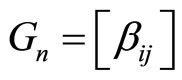 with elements
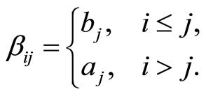 (1)
(1)
is given. On the other hand, the analytic expressions of the inverses of two symmetric matrices 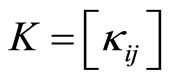 and
and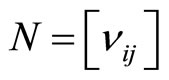 , where
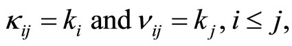 (2)
(2)
respectively, are presented in [2] (first equation in p. 113, and Equation (1), respectively). The matrix K is a special case of Brownian matrix and  is a lower Brownian matrix, as they have been defined in [3] (Equation (2.1)). Earlier, in [4] (paragraph following Equation (3.3)) the term “pure Brownian matrix” for the type of the matrix K has introduced. Furthermore, in [5] (discussion concerning Equations (28)-(30)) the so-called “diagonal innovation matrices” (DIM) have been treated, special cases of which are the matrices K and N.
In the present paper, we consider two matrices A1 and A2 defined by
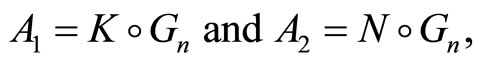 (3)
(3)
where the symbol  denotes the Hadamard product. Hence, the matrices have the forms
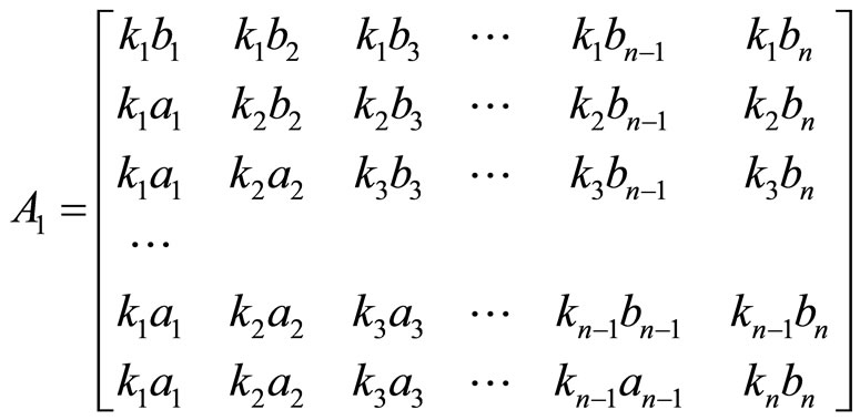 (4)
(4)
and
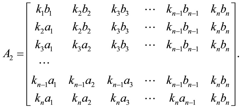 (5)
(5)
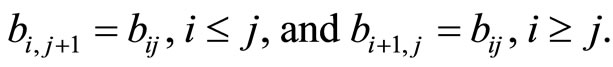
Let us now define for a matrix 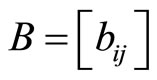 the terms “pure upper Brownian matrix” and “pure lower Brownian matrix”, for the elements of which the following relations are respectively valid
 (6)
(6)
The matrix A1 (Equation (4)) is a lower Brownian matrix. Furthermore, the matrix PNP, where  is the permutation matrix with elements
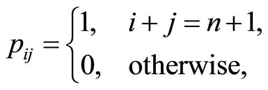 (7)
(7)
is a pure Brownian matrix and  a pure lower Brownian matrix. Hence, their Hadamard product
  gives a pure lower Brownian matrix, that is, the matrix
 .
.
In the following sections, we deduce in analytic form the inverses and determinants of the matrices A1 and A2; and we study the numerical complexity on evaluating  and
and .
.
2. The Inverse and Determinant of A1
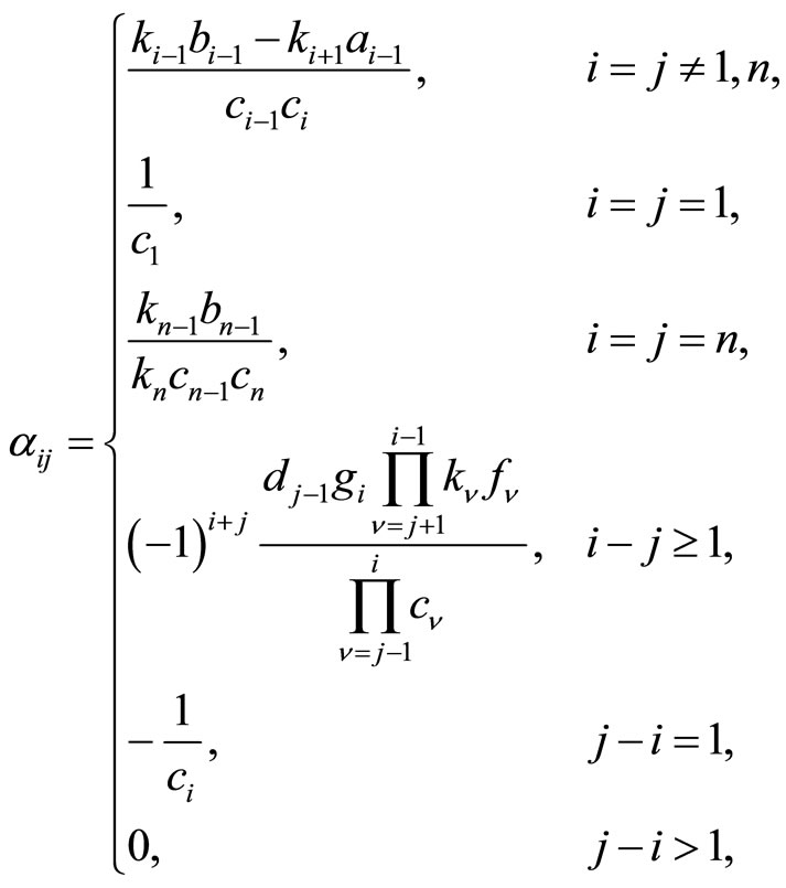
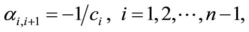
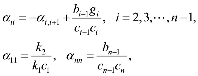
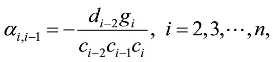
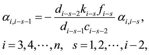
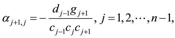
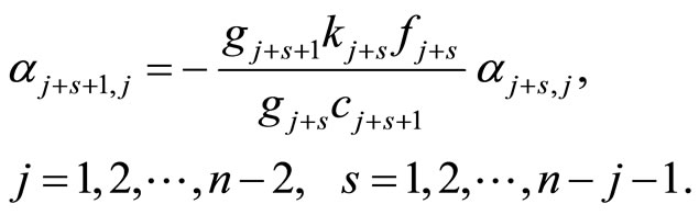
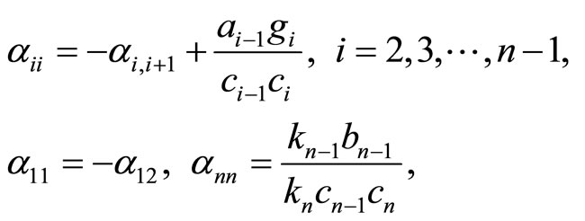
The inverse of A1 is a lower Hessenberg matrix expressed analytically by the 3n − 1 parameters defining A1. In particular, the inverse  has elements given by the relations
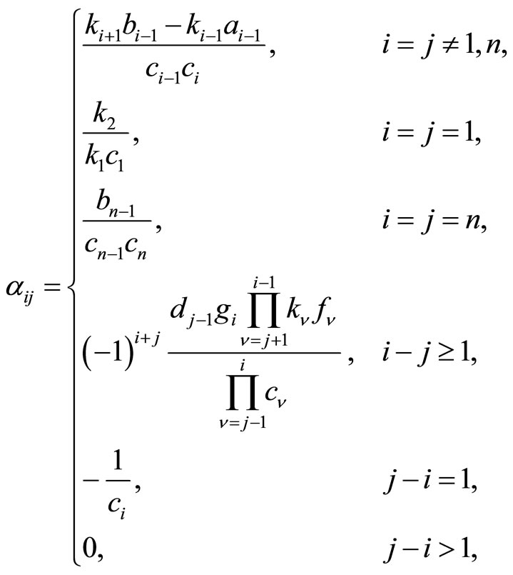 (8)
(8)
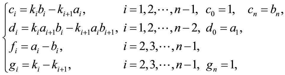
where
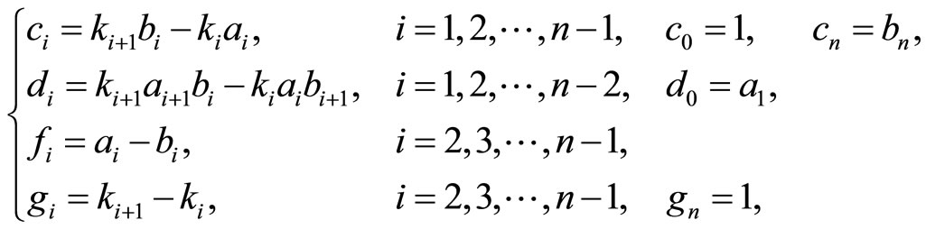 (9)
(9)
with
 (10)
(10)
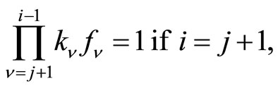
and with the obvious assumptions
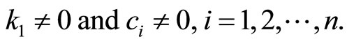 (11)
(11)
To prove that the relations (8)-(10) give the inverse matrix , we reduce A1 to the identity matrix I by applying a number of elementary row transformations.
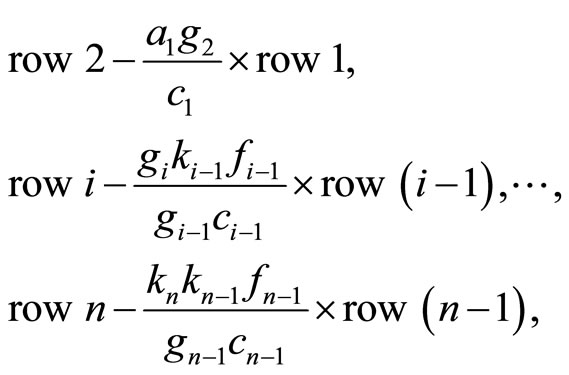
Then the product of the corresponding elementary matrices gives the inverse matrix of A1. These transformations are defined by the following sequence of row operations.
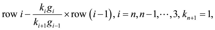
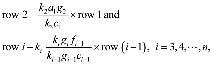
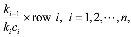
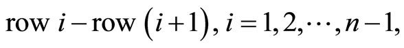
Operation 1 (applied on A1 and on the identity matrix I):

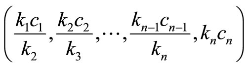
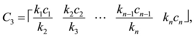
which transforms A1 into the lower triangular matrix C1 given by
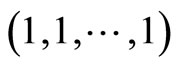
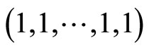
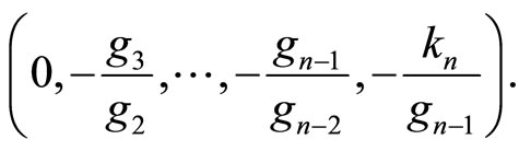
and the identity matrix I into the upper bidiagonal matrix F1 with main diagonal
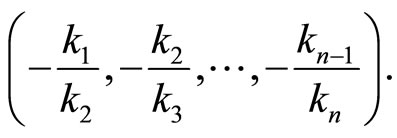
and upper first diagonal
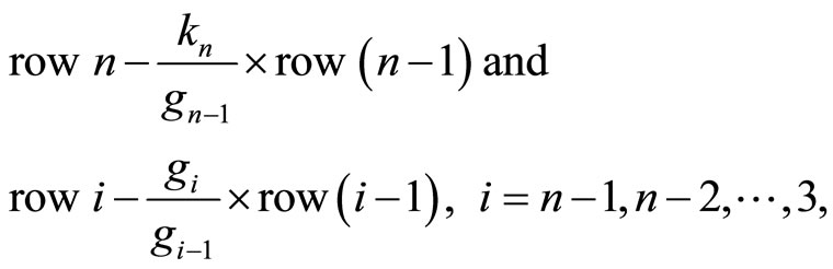
Operation 2 (applied on  and
and ):
):
which derives a lower bidiagonal matrix  with main diagonal
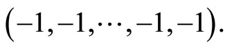
and lower first diagonal
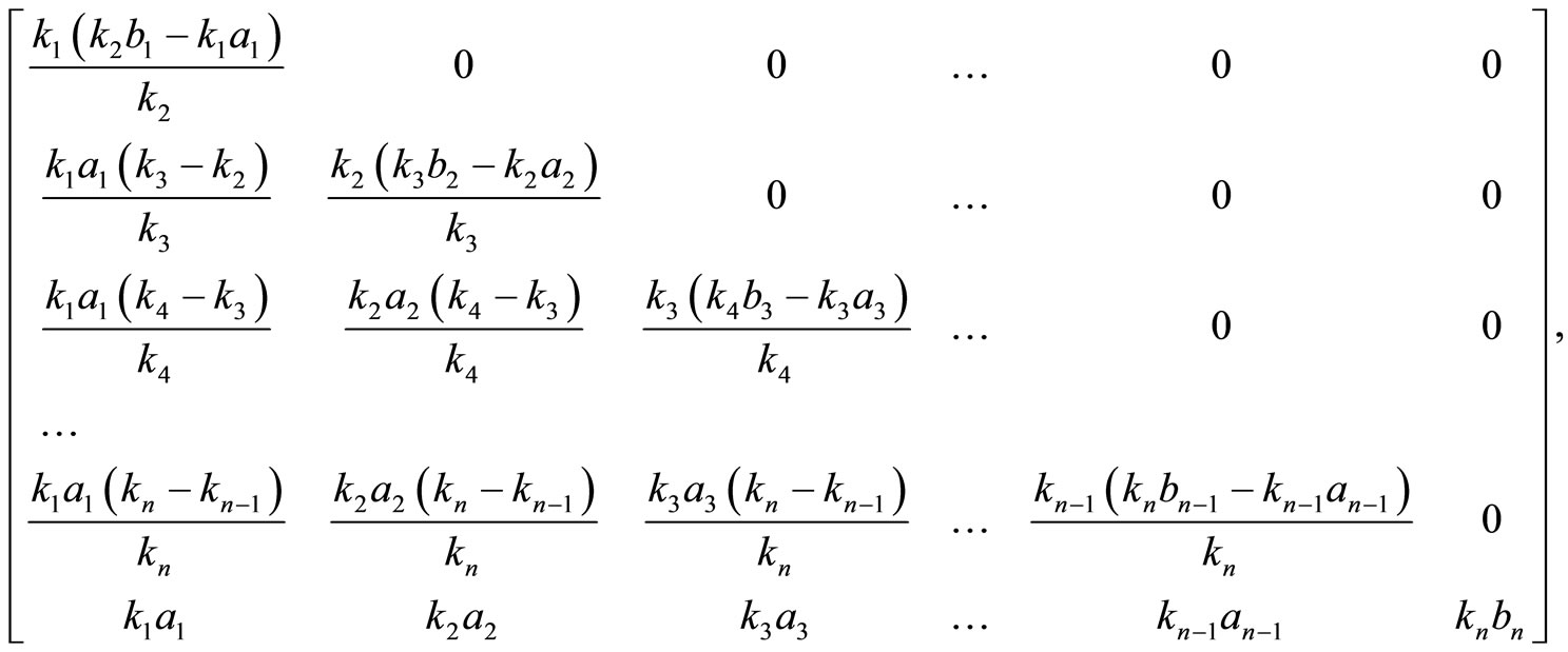
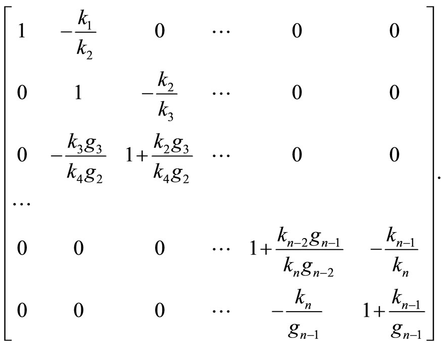
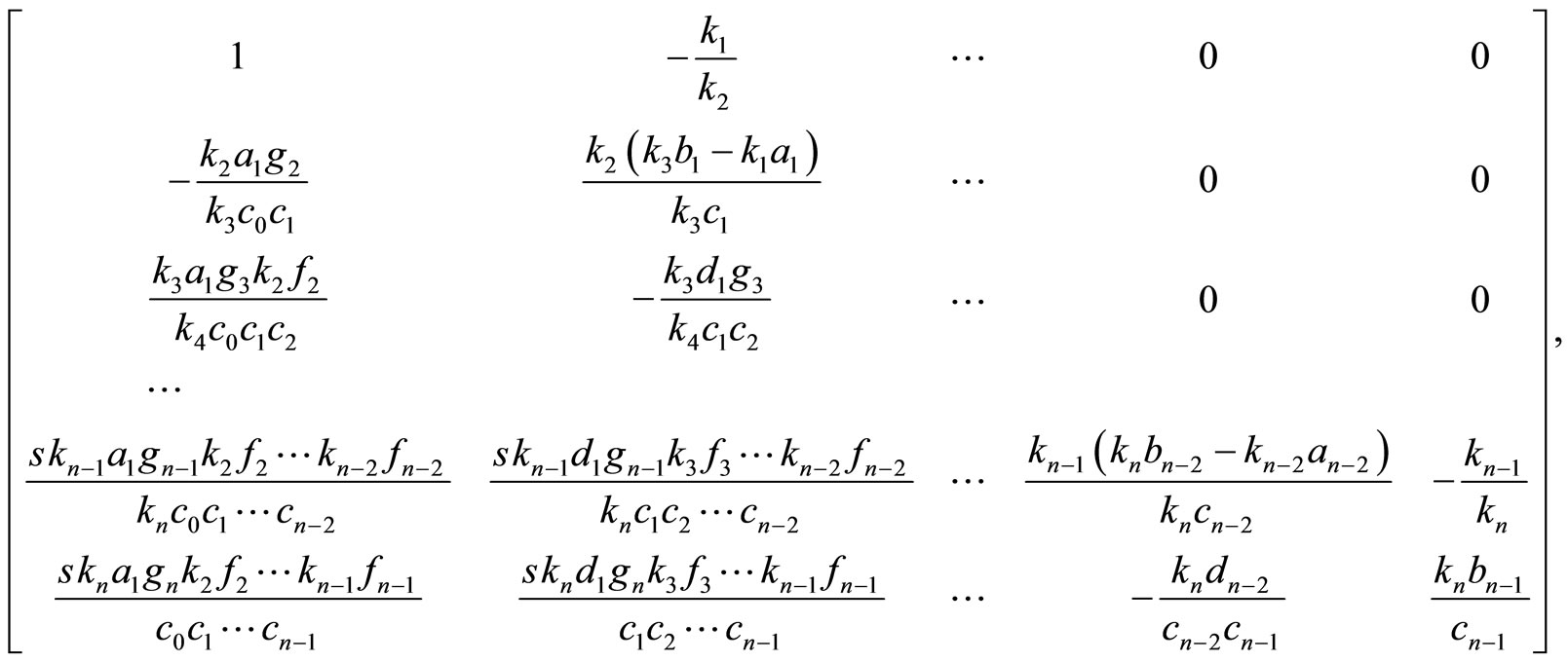
while the matrix  is transformed into the tridiagonal matrix
  given by
Operation 3 (applied on  and
and ):
):
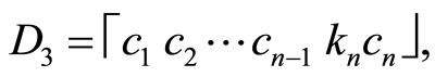
which derives the diagonal matrix
and, respectively, the lower Hessenberg matrix F3 given by
with the symbol s standing for the quantity .
.
Operation 4 (applied on  and
and ):
):
which transforms  into the identity matrix I and the matrix
  into the inverse
 .
.
The determinant of  takes the form
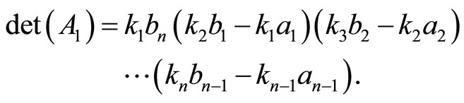 (12)
(12)
Evidently,  is singular if
  or, considering the relation (9), if
  for some
 .
.
3. The Inverse and Determinant of A2
In the case of , its inverse
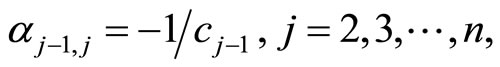
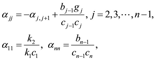
  is a lower Hessenberg matrix with elements given by the relations
 (13)
(13)
where
 (14)
(14)
with
 (15)
(15)
and with the obvious assumptions
 (16)
(16)
In order to prove that the relations (13)-(15) give the inverse matrix , we follow a similar manner to that of Section 2.
Operation 1 (applied on A2 and on the identity matrix I):
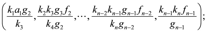
which transforms A2 into the lower triangular matrix  equal to

and the identity matrix I into the bidiagonal matrix  with main diagonal
and upper first diagonal
Operation 2 (applied on  and
and ):
):
which derives the lower bidiagonal matrix D2 with main diagonal
and lower first diagonal
while the matrix  is transformed into the tridiagonal matrix
  with main diagonal
upper first diagonal
and lower first diagonal
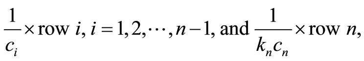
Operation 3 (applied on  and
and ):
):
with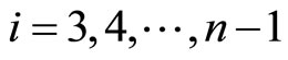 , which yields the diagonal matrix
 ,
,
and the lower Hessenberg matrix  equal to
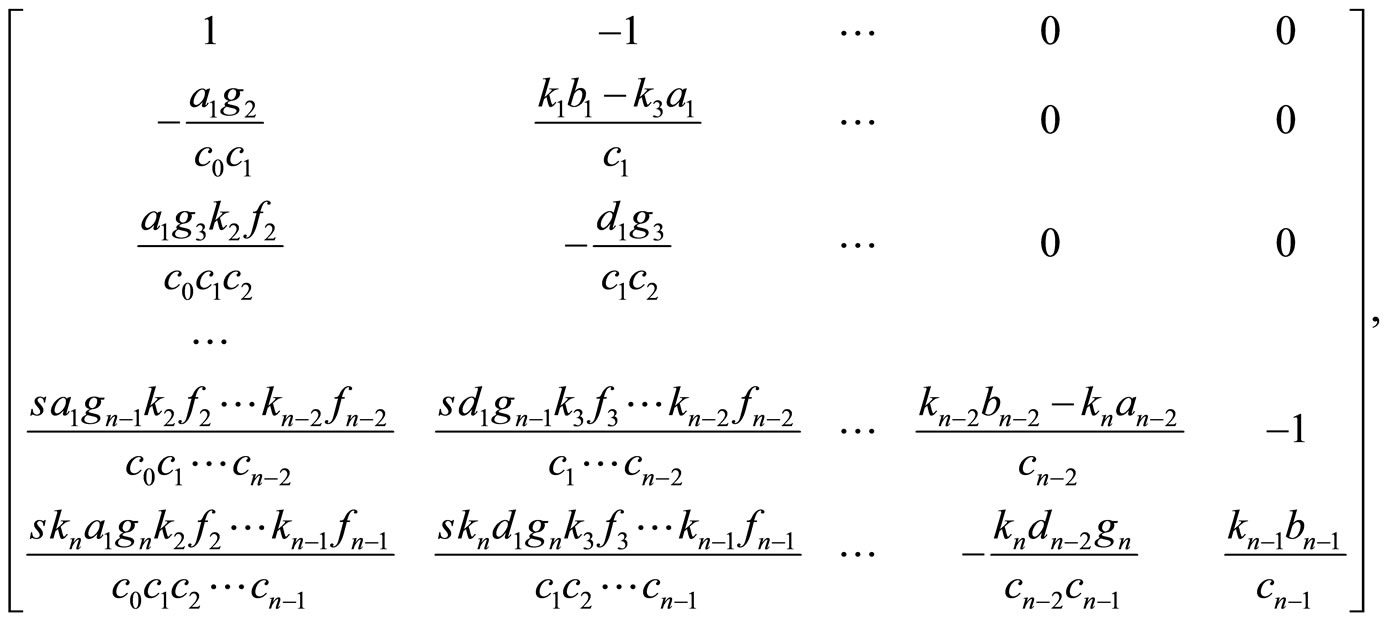
where the symbol  stands for
 .
.
Operation 4 (applied on  and
and ):
):
which transforms  into the identity matrix I and
  into the inverse
 .
.
The determinant of  has the form
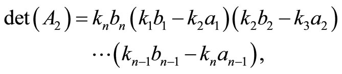 (17)
(17)
which shows in turn that the matrix  is singular if
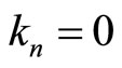 , or, adopting the conventions (14), if
  for some
 .
.
4. Numerical Complexity
The relations (8) and (13) lead to recurrence formulae, by which the inverses  and
and , respectively, are computed in
  multiplications/divisions and
  additions/substractions. In fact, the recursive algorithm
 (18)
(18)
 (19)
(19)
 (20)
(20)
 (21)
(21)
where ,
,  ,
,  , and
, and  are given by the relation (9), computes
  in
in 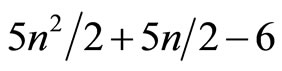 mult/div (since the coefficients of
  depends only on the second subscript) and
 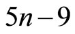 add/sub.
In terms of , the above algorithm takes the form
For the computation of  the algorithms (18)-(21) changes only in the estimation of the diagonal elements, for which we have
where ,
,  ,
,  , and
, and  are given by the relation (14). Therefore, considering the relations (9) and (14), it is clear that the number of mult/div and add/sub in computing
  is the same with that of
 .
.
5. Concluding Remarks
The matrices A1 and A2 represent generalizations of known classes of test matrices. For instance, the test matrices given in [6] (Equations (2.1) and (2.2)) and in [1] (Eq. (2)) belong to the categories presented. Furthermore, by restricting the a’s and b’s to unity, A1 and A2 reduce to the matrices given in [2]. Also, the matrices in [7] (pp. 41, 42, 49) are special cases of A1 and A2. On the other hand, concerning the recursive algorithms given in Section 4, we have performed numerical experiments by assigning random values to the parameters of A1, and with a variety of the order n from 256 to 1024. We have found that computing  by the recursive algorithms (18)-(21) is ~100 times faster than using the LU decomposition when n = 256 and increases gradually to ~1000 times faster when n = 1024.
REFERENCES
- R. J. Herbold, “A Generalization of a Class of Test Matrices,” Mathematics of Computation, Vol. 23, 1969, pp. 823-826. doi:10.1090/S0025-5718-1969-0258259-0
- F. N. Valvi, “Explicit Presentation of the Inverses of Some Types of Matrices,” IMA Journal of Applied Mathematics, Vol. 19, No. 1, 1977, pp. 107-117. doi:10.1093/imamat/19.1.107
- M. J. C. Gover and S. Barnett, “Brownian Matrices: Properties and Extensions,” International Journal of Systems Science, Vol. 17, No. 2, 1986, pp. 381-386. doi:10.1080/00207728608926813
- B. Picinbono, “Fast Algorithms for Brownian Matrices,” IEEE Transactions on Acoustics, Speech and Signal Processing, Vol. 31, No. 2, 1983, pp. 512-514. doi:10.1109/TASSP.1983.1164078
- G. Carayannis, N. Kalouptsidis and D. G. Manolakis, “Fast Recursive Algorithms for a Class of Linear Equations,” IEEE Transactions on Acoustics, Speech and Signal Processing, Vol. 30, No. 2, 1982, pp. 227-239. doi:10.1109/TASSP.1982.1163876
- H. W. Milnes, “A Note Concerning the Properties of a Certain Class of Test Matrices,” Mathematics of Computation, Vol. 22, 1968, pp. 827-832. doi:10.1090/S0025-5718-1968-0239743-1
- R. T. Gregory and D. L. Karney, “A Collection of Matrices for Testing Computational Algorithms,” Wiley-Interscience, London, 1969.